This notebook continues the opening chapter with a small toy dataset.
Toy sample
import numpy as np
import pandas as pd
import matplotlib.pyplot as plt

x = np.array([1.2, 0.7, 1.5, 2.1, 0.9, 1.8, 1.1, 1.4])
summary = pd.DataFrame({
    "observation": np.arange(1, len(x) + 1),
    "value": x,
})
summary
| 0 |
1 |
1.2 |
| 1 |
2 |
0.7 |
| 2 |
3 |
1.5 |
| 3 |
4 |
2.1 |
| 4 |
5 |
0.9 |
| 5 |
6 |
1.8 |
| 6 |
7 |
1.1 |
| 7 |
8 |
1.4 |
Sample moments
n = len(x)
xbar = x.mean()
m2 = np.mean((x - xbar) ** 2)
m3 = np.mean((x - xbar) ** 3)
m4 = np.mean((x - xbar) ** 4)

pd.DataFrame({
    "quantity": ["n", "xbar", "m2", "m3", "m4"],
    "value": [n, xbar, m2, m3, m4],
})
| 0 |
n |
8.000000 |
| 1 |
xbar |
1.337500 |
| 2 |
m2 |
0.187344 |
| 3 |
m3 |
0.023496 |
| 4 |
m4 |
0.073730 |
Quick plot
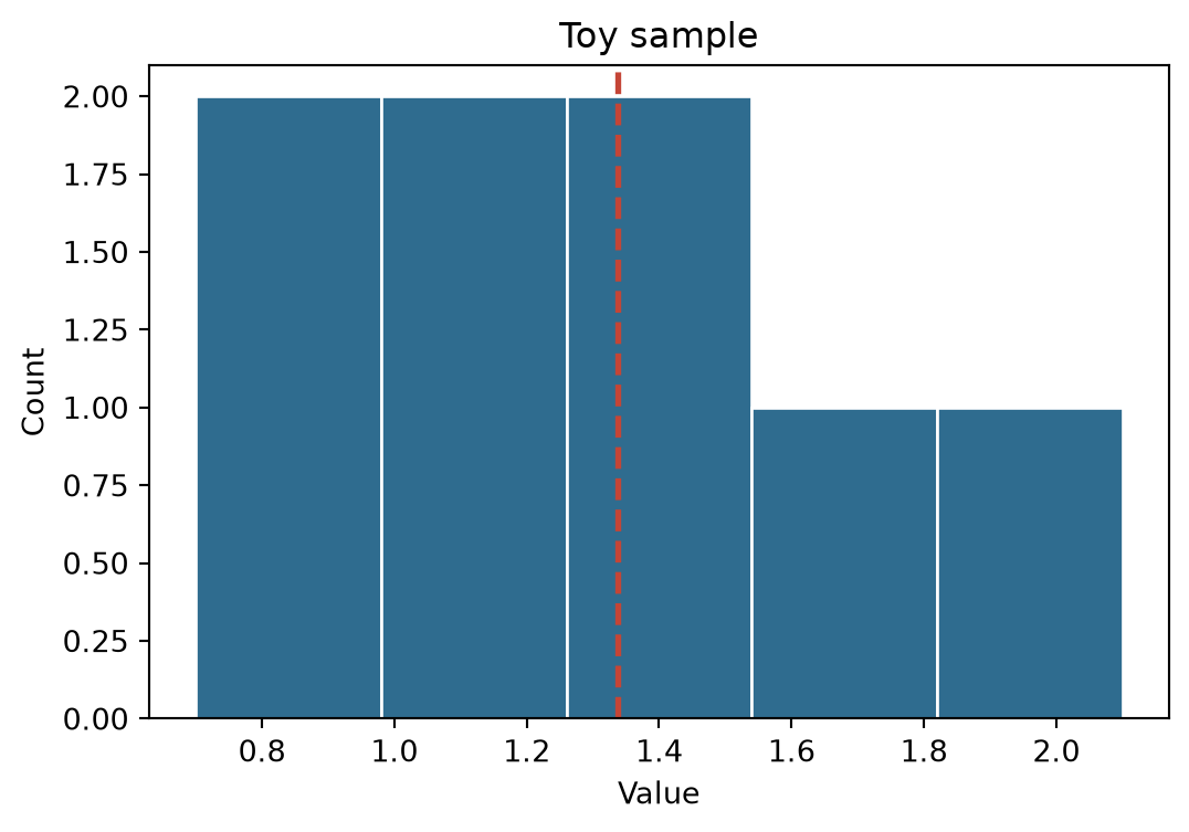
fig, ax = plt.subplots(figsize=(6.2, 4.0))
ax.hist(x, bins=5, color="#2f6c8f", edgecolor="white")
ax.axvline(xbar, color="#c44536", linestyle="--", linewidth=2)
ax.set_xlabel("Value")
ax.set_ylabel("Count")
ax.set_title("Toy sample")
plt.show()