{
const root = html`<div class="interference-widget">
<div class="interference-tabs" role="tablist" aria-label="Wave-packet explanation">
<button type="button" data-tab="0" role="tab" aria-selected="true">x packet</button>
<button type="button" data-tab="1" role="tab" aria-selected="false">motion</button>
<button type="button" data-tab="2" role="tab" aria-selected="false">velocity space</button>
<button type="button" data-tab="3" role="tab" aria-selected="false">interaction wave</button>
<button type="button" data-tab="4" role="tab" aria-selected="false">sum and drift</button>
</div>
<div class="interference-controls">
<label>
<span>charge product</span>
<select name="chargeProduct">
<option value="-1">q1 q2 < 0: attraction</option>
<option value="1">q1 q2 > 0: repulsion</option>
</select>
</label>
<label>
<span>mean velocity v0</span>
<input name="meanVelocity" type="range" min="-1.1" max="1.1" step="0.05" value="0">
<output></output>
</label>
</div>
<div class="interference-plot" aria-live="polite"></div>
</div>`;
const plot = root.querySelector(".interference-plot");
const buttons = Array.from(root.querySelectorAll("[data-tab]"));
const chargeProduct = root.querySelector("[name='chargeProduct']");
const meanVelocity = root.querySelector("[name='meanVelocity']");
const meanVelocityOut = meanVelocity.nextElementSibling;
const state = {tab: 0};
const width = 1120;
const height = 560;
const colors = {
axis: "#d7dde8",
grid: "#233044",
muted: "#9fb0c7",
initial: "#d7dde8",
interaction: "#58a6ff",
final: "#ffcc4d",
attraction: "#8ec5ff",
repulsion: "#ff9f5a",
constructive: "rgba(88, 166, 255, 0.16)",
destructive: "rgba(255, 117, 117, 0.14)"
};
const gaussian = (x, mu, sigma) => Math.exp(-0.5 * ((x - mu) / sigma) ** 2);
const interactionWave = (v, v0, direction) => {
const z = (v - v0) / 0.74;
return 0.48 * direction * z * Math.exp(-0.5 * z * z);
};
const resultWave = (v, v0, direction) => (
gaussian(v, v0, 0.82) + interactionWave(v, v0, direction)
);
const samplePath = (xmin, xmax, steps, sx, sy, fn) => {
let d = "";
for (let i = 0; i <= steps; i++) {
const x = xmin + (xmax - xmin) * i / steps;
d += `${i === 0 ? "M" : "L"} ${sx(x).toFixed(1)} ${sy(fn(x)).toFixed(1)} `;
}
return d;
};
const axis = ({left, top, plotWidth, plotHeight, xmin, xmax, ymin, ymax, xLabel, yLabel, ticks = [-3, -2, -1, 0, 1, 2, 3]}) => {
const sx = (x) => left + (x - xmin) / (xmax - xmin) * plotWidth;
const sy = (y) => top + (ymax - y) / (ymax - ymin) * plotHeight;
const xAxisY = sy(0);
const yAxisX = sx(0);
const grid = ticks.map((t) => `
<line x1="${sx(t)}" y1="${top}" x2="${sx(t)}" y2="${top + plotHeight}" class="interference-grid"/>
<text x="${sx(t)}" y="${top + plotHeight + 28}" class="interference-tick">${t}</text>
`).join("");
return {
sx,
sy,
markup: `
<rect x="${left}" y="${top}" width="${plotWidth}" height="${plotHeight}" class="interference-panel"/>
${grid}
<line x1="${left}" y1="${xAxisY}" x2="${left + plotWidth + 20}" y2="${xAxisY}" class="interference-axis" marker-end="url(#qi-arrow)"/>
<line x1="${yAxisX}" y1="${top + plotHeight}" x2="${yAxisX}" y2="${top - 16}" class="interference-axis" marker-end="url(#qi-arrow)"/>
<text x="${left + plotWidth}" y="${top + plotHeight + 58}" class="interference-axis-label">${xLabel}</text>
<text x="${yAxisX + 16}" y="${top + 18}" class="interference-axis-label">${yLabel}</text>
`
};
};
const defs = () => `
<defs>
<marker id="qi-arrow" markerWidth="9" markerHeight="9" refX="7" refY="4.5" orient="auto" markerUnits="strokeWidth">
<path d="M 0 0 L 9 4.5 L 0 9 Z" fill="${colors.axis}"/>
</marker>
<filter id="qi-glow" x="-60%" y="-60%" width="220%" height="220%">
<feGaussianBlur stdDeviation="5" result="blur"/>
<feMerge>
<feMergeNode in="blur"/>
<feMergeNode in="SourceGraphic"/>
</feMerge>
</filter>
</defs>
`;
const title = (main, sub) => `
<text x="56" y="48" class="interference-title">${main}</text>
<text x="56" y="82" class="interference-subtitle">${sub}</text>
`;
const svg = (body) => `
<svg viewBox="0 0 ${width} ${height}" role="img" aria-label="Wave-packet interference explanation">
${defs()}
<rect x="0" y="0" width="${width}" height="${height}" rx="16" class="interference-bg"/>
${body}
</svg>
`;
const tabXPacket = () => {
const ax = axis({left: 92, top: 122, plotWidth: 920, plotHeight: 320, xmin: -4, xmax: 4, ymin: -0.05, ymax: 1.18, xLabel: "position x", yLabel: "amplitude"});
const packet = samplePath(-4, 4, 220, ax.sx, ax.sy, (x) => gaussian(x, 0, 0.82));
return svg(`
${title("1. A localized wave packet", "In x-space the particle is represented by a wave packet, not by a point.")}
${ax.markup}
<path d="${packet}" class="interference-curve interference-initial interference-draw"/>
<line x1="${ax.sx(0)}" y1="${ax.sy(-0.02)}" x2="${ax.sx(0)}" y2="${ax.sy(1.04)}" class="interference-centerline"/>
<text x="${ax.sx(0) + 18}" y="${ax.sy(0.94)}" class="interference-label">center of the packet</text>
`);
};
const tabMotion = (v0) => {
const ax = axis({left: 92, top: 122, plotWidth: 920, plotHeight: 320, xmin: -4, xmax: 4, ymin: -0.05, ymax: 1.18, xLabel: "position x", yLabel: "amplitude"});
const shift = 1.5 * v0;
const initial = samplePath(-4, 4, 220, ax.sx, ax.sy, (x) => gaussian(x, 0, 0.82));
const moved = samplePath(-4, 4, 220, ax.sx, ax.sy, (x) => gaussian(x, shift, 0.82));
const label = v0 > 0.03 ? "<v> > 0" : (v0 < -0.03 ? "<v> < 0" : "<v> = 0");
return svg(`
${title("2. Motion is the drift of the packet", "Changing the mean velocity only shifts the packet center in time.")}
${ax.markup}
<path d="${initial}" class="interference-curve interference-ghost"/>
<path d="${moved}" class="interference-curve interference-final interference-slide"/>
<line x1="${ax.sx(0)}" y1="${ax.sy(0.42)}" x2="${ax.sx(shift)}" y2="${ax.sy(0.42)}" class="interference-arrow" marker-end="url(#qi-arrow)"/>
<text x="${ax.sx(shift) + (v0 >= 0 ? 18 : -18)}" y="${ax.sy(0.52)}" class="interference-label ${v0 >= 0 ? "" : "interference-label-left"}">${label}</text>
`);
};
const tabVelocity = (v0) => {
const ax = axis({left: 92, top: 122, plotWidth: 920, plotHeight: 320, xmin: -3.2, xmax: 3.2, ymin: -0.05, ymax: 1.18, xLabel: "velocity v", yLabel: "amplitude"});
const packet = samplePath(-3.2, 3.2, 220, ax.sx, ax.sy, (v) => gaussian(v, v0, 0.82));
return svg(`
${title("3. The same packet in velocity space", "A moving packet is a Gaussian shifted away from v = 0; its width stays fixed.")}
${ax.markup}
<path d="${packet}" class="interference-curve interference-initial interference-draw"/>
<line x1="${ax.sx(v0)}" y1="${ax.sy(-0.02)}" x2="${ax.sx(v0)}" y2="${ax.sy(1.02)}" class="interference-centerline"/>
<text x="${ax.sx(v0) + 18}" y="${ax.sy(0.92)}" class="interference-label">mean velocity v0 = ${v0.toFixed(2)}</text>
`);
};
const tabInteraction = (v0, direction, modeLabel) => {
const ax = axis({left: 92, top: 122, plotWidth: 920, plotHeight: 320, xmin: -3.2, xmax: 3.2, ymin: -0.55, ymax: 1.18, xLabel: "velocity v", yLabel: "amplitude"});
const incoming = samplePath(-3.2, 3.2, 240, ax.sx, ax.sy, (v) => gaussian(v, v0, 0.82));
const produced = samplePath(-3.2, 3.2, 240, ax.sx, ax.sy, (v) => interactionWave(v, v0, direction));
const plusSide = direction > 0 ? [v0, 3.2] : [-3.2, v0];
const minusSide = direction > 0 ? [-3.2, v0] : [v0, 3.2];
return svg(`
${title("4. The interaction creates an extra wave", `${modeLabel}: the produced wave has opposite signs on the two sides of the packet.`)}
${ax.markup}
<rect x="${ax.sx(plusSide[0])}" y="${ax.sy(1.16)}" width="${Math.abs(ax.sx(plusSide[1]) - ax.sx(plusSide[0]))}" height="${ax.sy(-0.52) - ax.sy(1.16)}" class="interference-constructive"/>
<rect x="${ax.sx(minusSide[0])}" y="${ax.sy(1.16)}" width="${Math.abs(ax.sx(minusSide[1]) - ax.sx(minusSide[0]))}" height="${ax.sy(-0.52) - ax.sy(1.16)}" class="interference-destructive"/>
<path d="${incoming}" class="interference-curve interference-ghost"/>
<path d="${produced}" class="interference-curve interference-interaction interference-draw"/>
<text x="${ax.sx(direction > 0 ? 1.85 : -1.85)}" y="${ax.sy(0.78)}" class="interference-label">constructive</text>
<text x="${ax.sx(direction > 0 ? -1.85 : 1.85)}" y="${ax.sy(-0.28)}" class="interference-label">destructive</text>
`);
};
const tabSum = (v0, direction, modeLabel) => {
const top = axis({left: 78, top: 102, plotWidth: 450, plotHeight: 210, xmin: -3.2, xmax: 3.2, ymin: -0.35, ymax: 1.24, xLabel: "velocity v", yLabel: "amplitude", ticks: [-3, -2, -1, 0, 1, 2, 3]});
const bottom = axis({left: 608, top: 102, plotWidth: 430, plotHeight: 210, xmin: -4, xmax: 4, ymin: -0.05, ymax: 1.18, xLabel: "position x", yLabel: "amplitude", ticks: [-4, -2, 0, 2, 4]});
const initialV = samplePath(-3.2, 3.2, 220, top.sx, top.sy, (v) => gaussian(v, v0, 0.82));
const producedV = samplePath(-3.2, 3.2, 220, top.sx, top.sy, (v) => interactionWave(v, v0, direction));
const finalV = samplePath(-3.2, 3.2, 220, top.sx, top.sy, (v) => resultWave(v, v0, direction));
const drift = 1.15 * (v0 + 0.48 * direction);
const initialX = samplePath(-4, 4, 220, bottom.sx, bottom.sy, (x) => gaussian(x, 0, 0.82));
const finalX = samplePath(-4, 4, 220, bottom.sx, bottom.sy, (x) => gaussian(x, drift, 0.82));
const signLabel = direction > 0 ? "<v> shifts to the right" : "<v> shifts to the left";
return svg(`
${title("5. The observed packet is the sum", `${modeLabel}: interference redistributes probability and shifts the packet center.`)}
${top.markup}
${bottom.markup}
<path d="${initialV}" class="interference-curve interference-ghost"/>
<path d="${producedV}" class="interference-curve interference-interaction"/>
<path d="${finalV}" class="interference-curve interference-final interference-draw"/>
<text x="${top.sx(-2.95)}" y="${top.sy(1.1)}" class="interference-label">incoming + produced</text>
<path d="${initialX}" class="interference-curve interference-ghost"/>
<path d="${finalX}" class="interference-curve interference-final interference-slide"/>
<line x1="${bottom.sx(0)}" y1="${bottom.sy(0.38)}" x2="${bottom.sx(drift)}" y2="${bottom.sy(0.38)}" class="interference-arrow" marker-end="url(#qi-arrow)"/>
<text x="${bottom.sx(drift) + (direction > 0 ? 18 : -18)}" y="${bottom.sy(0.5)}" class="interference-label ${direction > 0 ? "" : "interference-label-left"}">${signLabel}</text>
<text x="80" y="474" class="interference-summary">The force is not inserted as a Newtonian push. It appears as a phase-sensitive sum of waves.</text>
`);
};
function render() {
const v0 = Number(meanVelocity.value);
const q12 = Number(chargeProduct.value);
const direction = q12 < 0 ? 1 : -1;
const modeLabel = q12 < 0 ? "attraction" : "repulsion";
meanVelocityOut.textContent = v0.toFixed(2);
buttons.forEach((button, index) => button.setAttribute("aria-selected", String(index === state.tab)));
if (state.tab === 0) plot.innerHTML = tabXPacket();
if (state.tab === 1) plot.innerHTML = tabMotion(v0);
if (state.tab === 2) plot.innerHTML = tabVelocity(v0);
if (state.tab === 3) plot.innerHTML = tabInteraction(v0, direction, modeLabel);
if (state.tab === 4) plot.innerHTML = tabSum(v0, direction, modeLabel);
}
buttons.forEach((button) => {
button.addEventListener("click", () => {
state.tab = Number(button.dataset.tab);
render();
});
});
chargeProduct.addEventListener("change", render);
meanVelocity.addEventListener("input", render);
render();
return root;
}Attraction and Repulsion in Quantum Field Theory
R. Feynman: Not every simple question can be answered simply.
2026-07-01
What this lecture is based on
- V. A. Allahverdyan and D. V. Naumov, notes on attraction and repulsion in scalar QED (paper to be published).
- D. V. Naumov, Quantum Field Theory for Experimentalists and Not Only. https://neutrinohit.github.io/books.html
- Slides: https://neutrinohit.github.io/qft-lectures/en/slides/ScalarQEDAttractionRepulsion.html
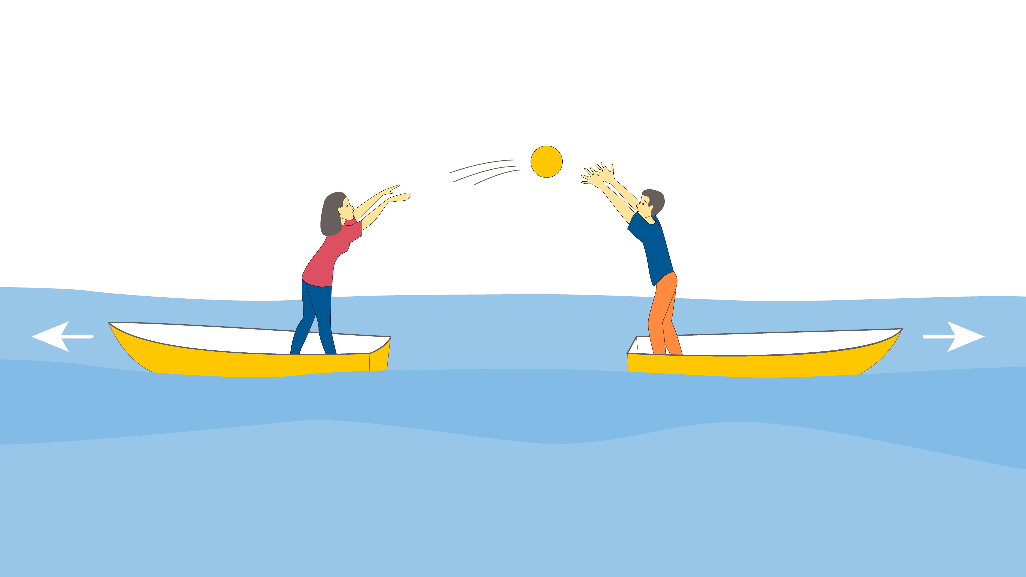
Repulsion picture: looks reasonable?
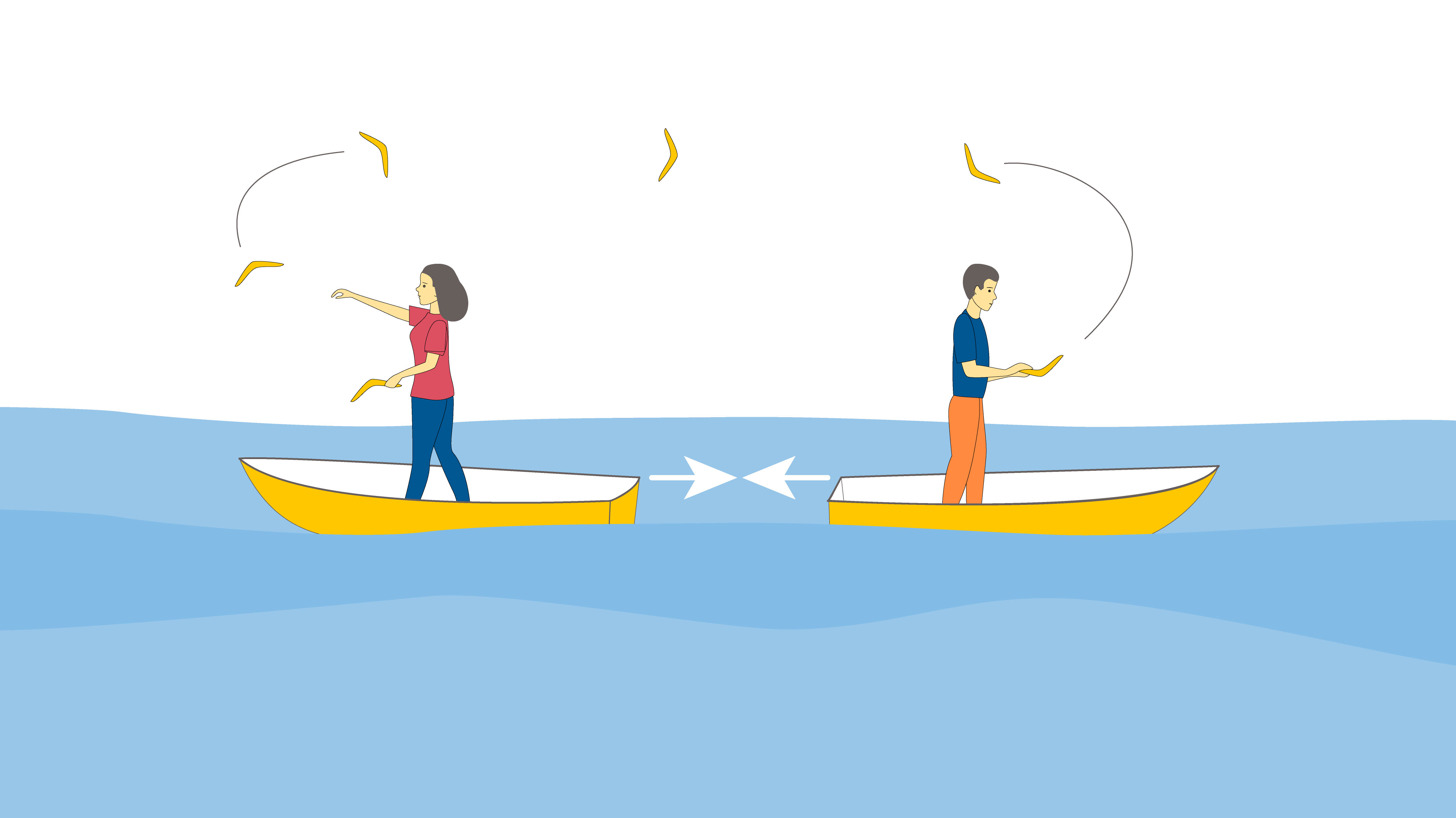
Attraction picture: looks reasonable too?
Zero order for \(\varphi\) and first order for \(A_\mu\)
- Narrow momentum packet
- Coordinate-space form
- Density and current
- Almost electrostatic
- Smoothed Coulomb kernel
- Profile of the kernel
- Laboratory system
- Animation
- In the packet rest frame, take \[ \widetilde\psi(\mathbf k) = (2\pi)^{3/4}\sigma_p^{-3/2} \exp\!\left[-\frac{\mathbf k^2}{4\sigma_p^2}\right], \qquad \sigma_p\ll m . \]
- The exact free solution is \[ \varphi_{\rm rest}^{(0)}(x) = \int\frac{d^3k}{(2\pi)^3} \widetilde\psi(\mathbf k) e^{i\mathbf k\cdot\mathbf x-iE_{\mathbf k}t}, \qquad E_{\mathbf k}=\sqrt{m^2+\mathbf k^2}. \]
Using
\[ E_{\mathbf k} =m+\frac{\mathbf k^2}{2m} +O\!\left(\frac{\sigma_p^4}{m^3}\right), \]
the packet is approximately
\[ \varphi_{\rm rest}^{(0)}(x) \approx \left(\frac{2\sigma_p^2}{\pi}\right)^{3/4} \frac{1}{(1+i\tau)^{3/2}} \exp\!\left[-\frac{\sigma_p^2\mathbf x^2}{1+i\tau}\right] e^{-imt}, \]
\[ \tau=\frac{2\sigma_p^2t}{m}, \qquad t_{\rm disp}=\frac{m}{2\sigma_p^2}. \]
Define
\[ s_p(t)=\frac{\sigma_p}{\sqrt{1+\tau^2}}, \qquad \sigma_x(t)=\frac{1}{2s_p(t)}. \]
Then
\[ n(t,\mathbf x)=|\varphi_{\rm rest}^{(0)}(x)|^2 = \left(\frac{2s_p^2(t)}{\pi}\right)^{3/2} \exp[-2s_p^2(t)\mathbf x^2]. \]
To leading order in \(\sigma_p/m\),
\[ J^\mu(t,\mathbf x) \approx \left( 2mn(t,\mathbf x), \; 4\frac{\sigma_p^2\tau}{1+\tau^2}\mathbf x\,n(t,\mathbf x) \right). \]
The spatial current is suppressed by \(\sigma_p/m\), so
\[ A_{\rm rest}^{(1)i}=O\!\left(\frac{\sigma_p}{m}\right), \qquad -\Delta A_{\rm rest}^{(1)0}(t,\mathbf x)\approx J^0(t,\mathbf x). \]
Thus
\[ A_{\rm rest}^{(1)0}(t,\mathbf x) \approx 2m\int d^3y\, \frac{n(t,\mathbf y)}{4\pi|\mathbf x-\mathbf y|}. \]
A finite packet replaces the point Coulomb source by a smooth charge cloud.
For a Gaussian packet,
\[ \boxed{ A_{\rm rest}^{(1)0}(t,r) \approx \frac{m}{2\pi r} \operatorname{erf}\!\left(\sqrt{2}\,s_p(t)r\right) } \]
or
\[ A_{\rm rest}^{(1)0}(t,r) \approx 2mV_{s_p(t)}(r), \qquad V_s(r)= \frac{1}{4\pi r} \operatorname{erf}\!\left(\sqrt{2}sr\right). \]
At large distance this is Coulomb. At the center it is finite.
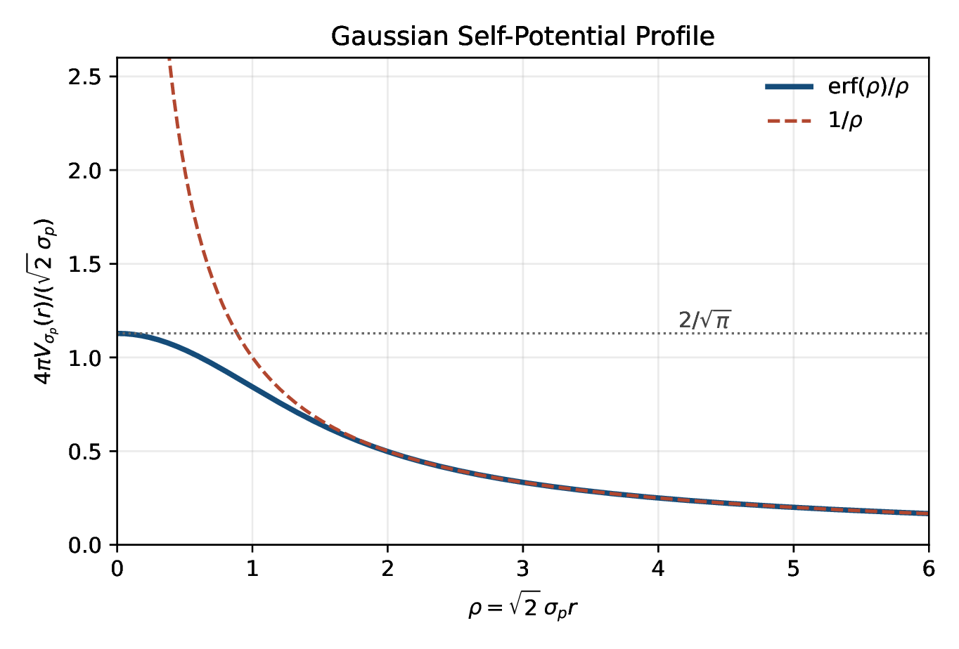
Dimensionless profile \(4\pi V_s(r)/(\sqrt{2}s)\) as a function of \(\rho=\sqrt{2}sr\). The dashed curve is the point Coulomb limit \(1/\rho\).
For a moving packet with mean four-momentum \(p_0^\mu=(E_0,\mathbf p_0)\),
\[ \mathbf v_0=\frac{\mathbf p_0}{E_0}, \qquad \gamma_0=\frac{E_0}{m}, \qquad \mathbf R=\mathbf x-\mathbf v_0t, \]
\[ t_*=\gamma_0(t-\mathbf v_0\cdot\mathbf x)=\frac{p_0\cdot x}{m}, \]
\[ r_*^2 = |\mathbf R|^2+ (\gamma_0^2-1)(\hat{\mathbf v}_0\cdot\mathbf R)^2. \]
Then
\[ \boxed{ A^{(1)\mu}(x) \approx 2p_0^\mu V_{s_p(t_*)}(r_*) }. \]
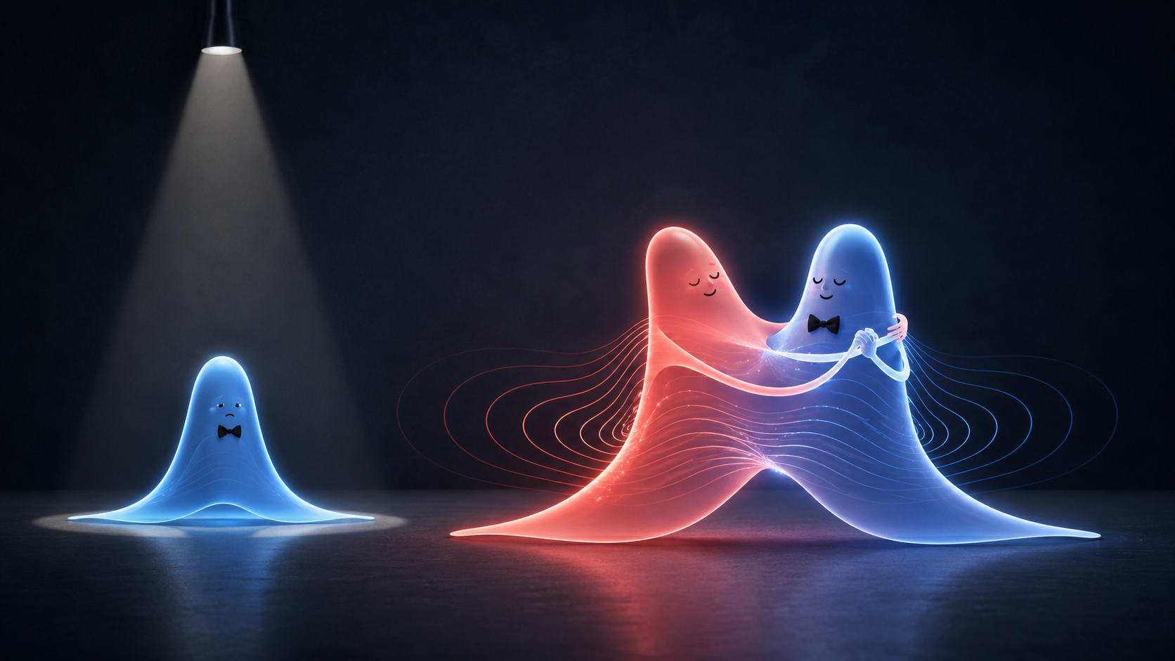
A lonely packet has no opinion
For one packet, the correction knows only \[ q^2 . \]
So the packet can acquire a self-phase, but it cannot decide whether the world is attractive or repulsive. \[ q \to -q \qquad\Rightarrow\qquad q^2 \to q^2 . \]
To ask about attraction or repulsion, we need a second packet.
The chain of ideas
The exchange picture is familiar. The question is sharper: where does the sign of attraction or repulsion enter?
The analogy changes the mechanism between the two cases. Scalar QED does not.
\[ \Psi(p,t)=\Phi(p)e^{-ipR}+\Delta\Psi(p,t) \]
\[ |\Psi|^2 = |\Phi|^2 +2\,\mathrm{Re}\!\left[\Phi^*(p)e^{ipR}\Delta\Psi(p,t)\right] +|\Delta\Psi|^2 \]
Like charges: the centers bend apart.
Opposite charges: the same construction bends them together.