Masterclass 2: Oscillations and Fit

SK-like spectrum with PEANUTS survival probabilities

Dmitry V. Naumov

JINR

2026-06-01

Lesson Map

• Tasks
• Inputs
• Oscillation Model
• Event Rate
• Pseudo-Data
• Fit
• Day-Night Optional
• Homework

Tasks

Goal for This Session

Masterclass 1 built the no-oscillation chain:

\[ \Phi_{^8\mathrm{B}} f_{^8\mathrm{B}}(E_\nu) \to \frac{dN}{dT_e}. \]

Today we add oscillations and fit two parameters:

\[ \Phi_{^8\mathrm{B}} f_{^8\mathrm{B}}(E_\nu) \to P_{ee}(E_\nu) \to \mu_j(\theta) \to n_j \to q(\theta). \]

Fit Parameters

Use

\[ \theta = \left( \sin^2\theta_{12}, \Delta m^2_{21} \right). \]

The main fit keeps the \(^8\mathrm{B}\) normalization fixed:

\[ \alpha_B=1. \]

The floating-normalization case is a homework extension.

Main Output

The notebook must produce:

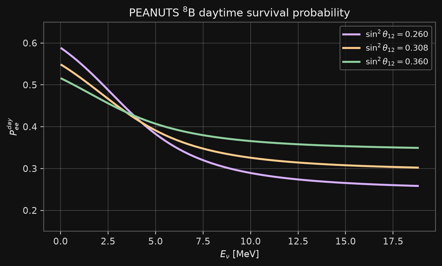
• \(P_{ee}^{day}(E_\nu)\) for several parameter points;
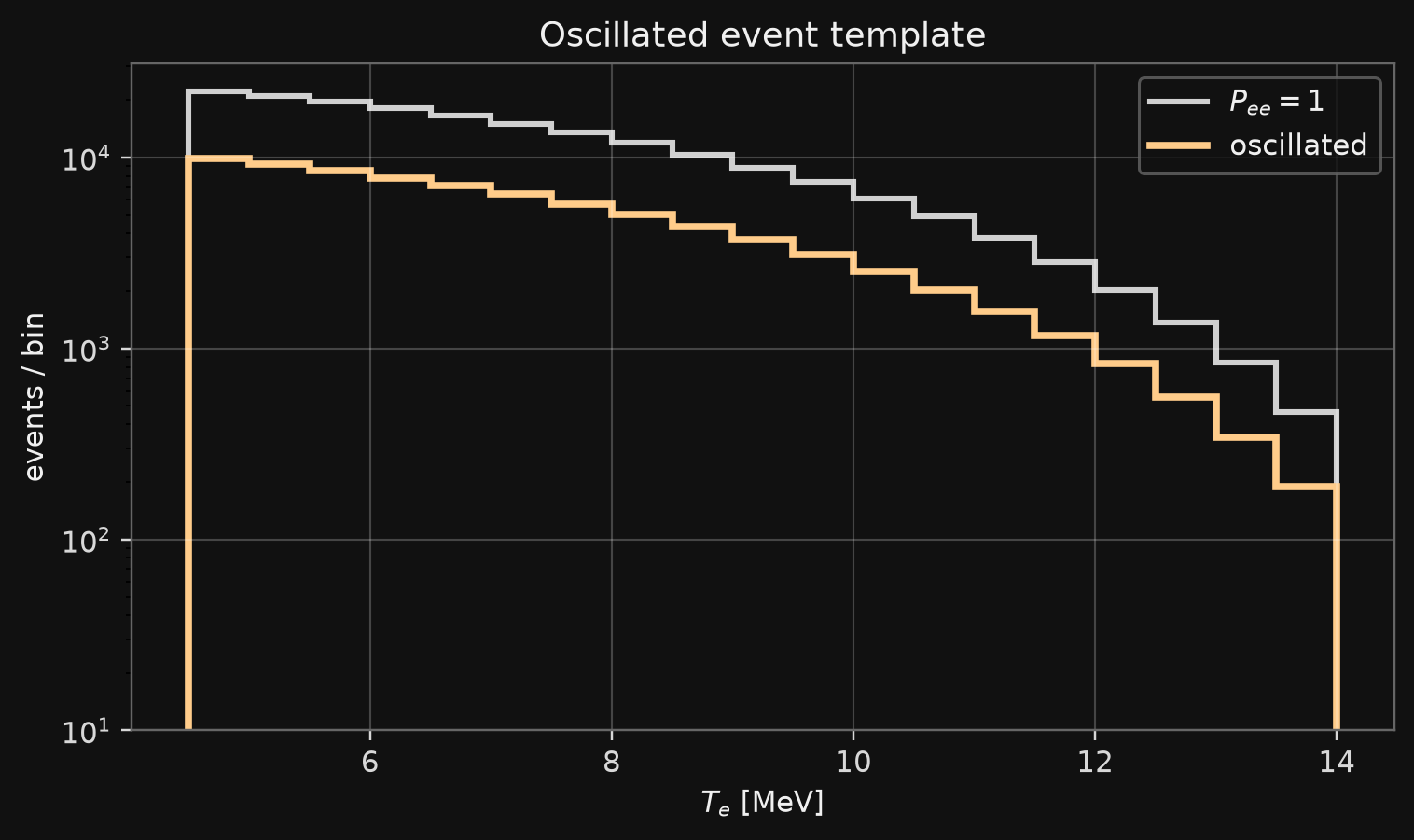
• oscillated SK-like recoil spectrum;
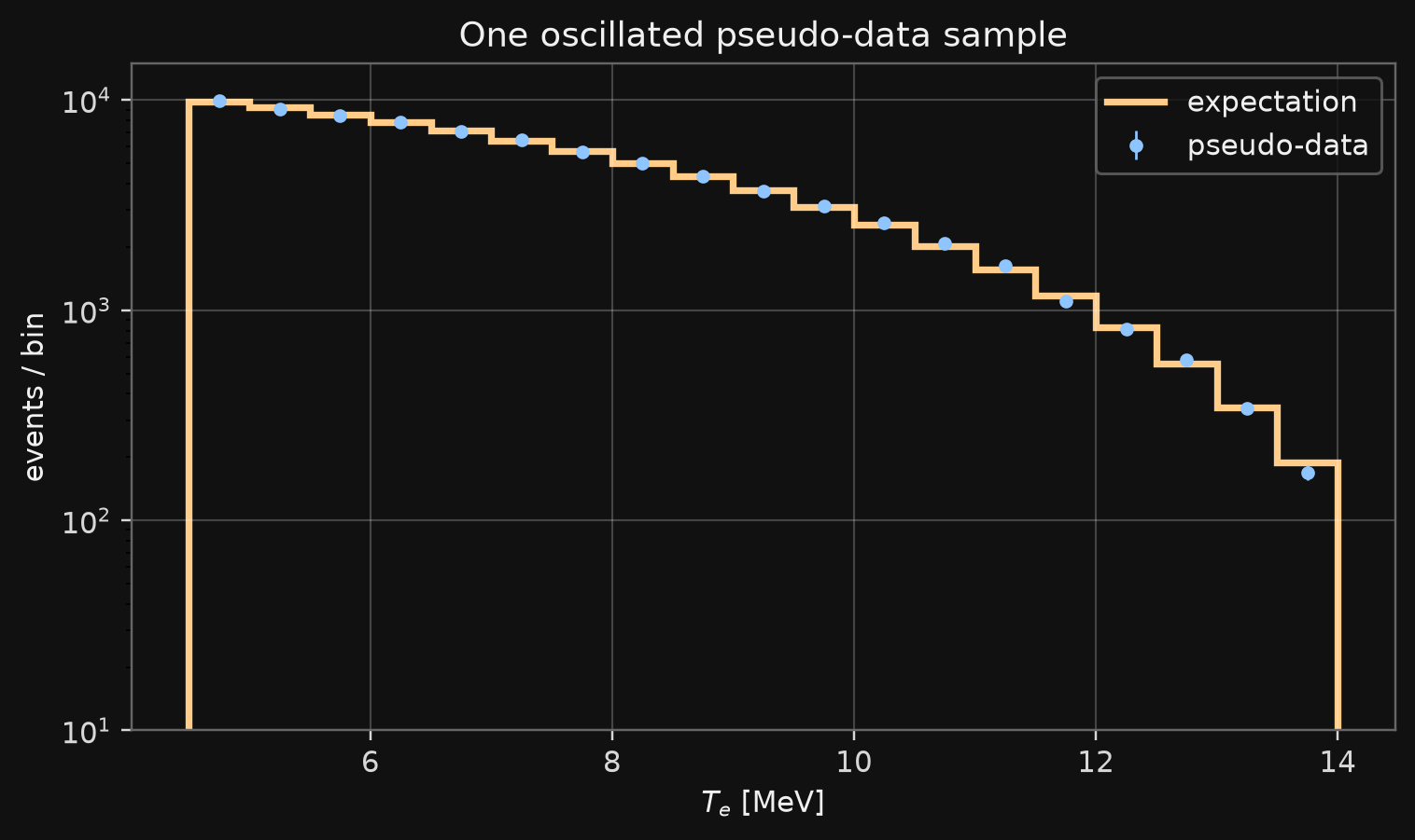
• pseudo-data in recoil-energy bins;
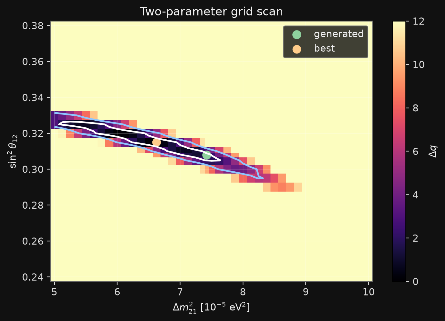
• best-fit point in \((\sin^2\theta_{12},\Delta m^2_{21})\);
• 2D contour and 1D profile checks.

Inputs

Project Page

Project page:

https://neutrinohit.github.io/neutrinophysics/
solar-neutrino-masterclass/

Tables used today:

data/masterclass2/solar_fluxes.csv
data/masterclass2/energy_spectra.csv
data/masterclass2/nu_electron_recoil_cross_sections.csv
data/masterclass2/oscillation_probabilities_grid.csv
data/masterclass2/earth_regeneration_grid.csv
data/masterclass2/earth_regeneration_parameter_scan.csv

Load the Tables

import numpy as np
import pandas as pd

BASE = "https://neutrinohit.github.io/neutrinophysics/solar-neutrino-masterclass"

fluxes = pd.read_csv(f"{BASE}/data/masterclass2/solar_fluxes.csv")
spectra = pd.read_csv(f"{BASE}/data/masterclass2/energy_spectra.csv")
xs = pd.read_csv(f"{BASE}/data/masterclass2/nu_electron_recoil_cross_sections.csv")
osc = pd.read_csv(f"{BASE}/data/masterclass2/oscillation_probabilities_grid.csv")
earth = pd.read_csv(f"{BASE}/data/masterclass2/earth_regeneration_grid.csv")
earth_scan = pd.read_csv(f"{BASE}/data/masterclass2/earth_regeneration_parameter_scan.csv")

The same archive is also available as:

data/masterclass2/masterclass2_data.zip

PEANUTS Grids

The oscillation tables are not analytic approximations.

They were generated with PEANUTS for \(^8\mathrm{B}\) neutrinos:

• oscillation_probabilities_grid.csv: \(P_{ee}^{day}(E_\nu;\sin^2\theta_{12},\Delta m^2_{21})\);
• earth_regeneration_grid.csv: \(P_{ee}^{night}(E_\nu,\eta)-P_{ee}^{day}(E_\nu)\) at reference parameters;
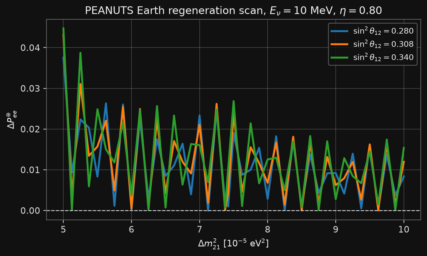
• earth_regeneration_parameter_scan.csv: the same Earth correction at selected \(E_\nu\) and \(\eta\) values while scanning \((\sin^2\theta_{12},\Delta m^2_{21})\);

The day-night material is optional today.

Details are in the lecture appendix:

Earth Matter appendix

Grid Check

Required columns:

E_MeV
sin2theta12
dm21_eV2
Pee_day

Expected checks:

print(len(osc), len(earth), len(earth_scan))
print(osc["sin2theta12"].min(), osc["sin2theta12"].max())
print(osc["dm21_eV2"].min(), osc["dm21_eV2"].max())

236880 1504 18900
0.24 0.38
5.0e-05 0.0001

Oscillation Model

Daytime Survival Probability

Use the PEANUTS table as a function:

\[ P_{ee}^{day} = P_{ee}^{day} \left( E_\nu;\sin^2\theta_{12},\Delta m^2_{21} \right). \]

Select a Parameter Point

Reference point:

\[ \sin^2\theta_{12}=0.308, \qquad \Delta m^2_{21}=7.42\times10^{-5}\ \mathrm{eV^2}. \]

sin2_ref = 0.308
dm21_ref = 7.42e-5

pee_ref_table = osc[
    np.isclose(osc["sin2theta12"], sin2_ref)
    & np.isclose(osc["dm21_eV2"], dm21_ref)
].sort_values("E_MeV")

Interpolate \(P_{ee}\)

The cross-section table is rectangular in \((E_\nu,T_e)\).

Interpolate \(P_{ee}\) onto the same \(E_\nu\) rows:

pee = np.interp(
    xs["E_MeV"],
    pee_ref_table["E_MeV"],
    pee_ref_table["Pee_day"],
    left=pee_ref_table["Pee_day"].iloc[0],
    right=pee_ref_table["Pee_day"].iloc[-1],
)

Check:

print(pee.min(), pee.max())

Effective Cross Section

The detector sees recoil electrons.

For each row \((E_\nu,T_e)\) use

\[ \frac{d\sigma_{\mathrm{eff}}}{dT_e} = P_{ee}\frac{d\sigma_{\nu_e e}}{dT_e} + (1-P_{ee})\frac{d\sigma_{\nu_x e}}{dT_e}. \]

Here \(\nu_x\) means \(\nu_\mu\) or \(\nu_\tau\).

The \(\nu_e e\) cross section is larger because it has both charged-current and neutral-current contributions. The coupling constants are summarized in the appendix:

Elastic Scattering Cross Section

Event Rate

Prediction Formula

For recoil-energy bin \(j\),

\[ \mu_j(\theta) = N_eT_{\rm live} \int_{T_j}^{T_{j+1}} dT_e \int dE_\nu\, \Phi_{^8\mathrm{B}}f_{^8\mathrm{B}}(E_\nu) \frac{d\sigma_{\mathrm{eff}}}{dT_e}. \]

In the table calculation, this is again a sum of row weights.

Build the Template

phi_b8 = float(fluxes.loc[fluxes["source"] == "B8", "flux_cm2_s"].iloc[0])
b8 = spectra.loc[spectra["source"] == "B8"].sort_values("E_MeV")

shape = np.interp(xs["E_MeV"], b8["E_MeV"], b8["spectrum_per_MeV"], left=0.0, right=0.0)
xs = xs.assign(dphi_dE=phi_b8 * shape)

effective_xs = (
    pee * xs["dsigma_nue_cm2_per_MeV"]
    + (1.0 - pee) * xs["dsigma_nux_cm2_per_MeV"]
)

Bin the Template

N_A = 6.02214076e23
seconds_per_year = 365.25 * 24 * 3600
N_e = 10.0 * N_A * 100.0e9 / 18.0
T_live = seconds_per_year

E_grid = np.sort(xs["E_MeV"].unique())
T_grid = np.sort(xs["T_e_MeV"].unique())
dE = np.median(np.diff(E_grid))
dT = np.median(np.diff(T_grid))

edges = np.arange(4.5, 14.0 + 0.25, 0.5)
bin_id = np.digitize(xs["T_e_MeV"], edges) - 1
valid = (0 <= bin_id) & (bin_id < len(edges) - 1)

Bin the Template

weights = (
    N_e * T_live
    * xs["dphi_dE"]
    * effective_xs
    * dE * dT
)

m = np.bincount(
    bin_id[valid],
    weights=weights[valid],
    minlength=len(edges) - 1,
)

Prediction Function

Use one function for every parameter point:

def prediction_from_pee(pee):
    effective_xs = (
        pee * xs["dsigma_nue_cm2_per_MeV"]
        + (1.0 - pee) * xs["dsigma_nux_cm2_per_MeV"]
    )
    weights = (
        N_e * T_live
        * xs["dphi_dE"]
        * effective_xs
        * dE * dT
    )
    return np.bincount(
        bin_id[valid],
        weights=weights[valid],
        minlength=len(edges) - 1,
    )

m = prediction_from_pee(pee)
m_noosc = prediction_from_pee(np.ones_like(pee))

Template Checks

Expected checks:

no-oscillation total = 186693.543
oscillated expected total = 80130.365

Plot the Template

The oscillated spectrum is lower than the no-oscillation spectrum, but not simply by a constant factor.

That shape difference is what the fit uses.

Expected first bins:

4.5 5.0 9863.1
5.0 5.5 9211.5
5.5 6.0 8534.9

Pseudo-Data

Generate Pseudo-Data

Generate counts in the same bins:

rng = np.random.default_rng(24680)
n = rng.poisson(m)
print(m.sum(), n.sum())

Expected output:

80130.365 79968

Use the same binning for data and prediction.

Do not rebin after generating pseudo-data.

Fit

Poisson Statistic

For a parameter point \(\theta\) compute \(\mu_j(\theta)\).

Use

\[ q(\theta) = 2\sum_j \left[ \mu_j(\theta)-n_j + n_j\ln\frac{n_j}{\mu_j(\theta)} \right]. \]

Then subtract the minimum:

\[ \Delta q(\theta)=q(\theta)-q_{\min}. \]

def poisson_q(n, mu):
    mu = np.maximum(mu, 1e-300)
    terms = mu.copy()
    mask = n > 0
    terms[mask] = mu[mask] - n[mask] + n[mask] * np.log(n[mask] / mu[mask])
    return 2.0 * np.sum(terms)

Grid Scan

Loop over the PEANUTS grid:

scan_rows = []

for sin2 in np.sort(osc["sin2theta12"].unique()):
    for dm21 in np.sort(osc["dm21_eV2"].unique()):
        table = osc[
            np.isclose(osc["sin2theta12"], sin2)
            & np.isclose(osc["dm21_eV2"], dm21)
        ].sort_values("E_MeV")

        pee = np.interp(xs["E_MeV"], table["E_MeV"], table["Pee_day"])
        mu = prediction_from_pee(pee)
        q = poisson_q(n, mu)
        scan_rows.append((sin2, dm21, q))

Best Fit

scan = pd.DataFrame(scan_rows, columns=["sin2theta12", "dm21_eV2", "q"])
scan["Delta_q"] = scan["q"] - scan["q"].min()

best = scan.loc[scan["q"].idxmin()]
print(best)

Expected output for the supplied pseudo-data:

best sin2theta12 = 0.31500
best dm21 = 6.625000e-05 eV^2

The generated point is still

\[ \sin^2\theta_{12}=0.308, \qquad \Delta m^2_{21}=7.42\times10^{-5}\ \mathrm{eV^2}. \]

Two-Dimensional Contour

For two fitted parameters, draw:

\[ \Delta q = 2.30, \qquad \Delta q = 6.18. \]

For the supplied pseudo-data, the approximate \(68\%\) grid range is:

sin2theta12 = 0.305 ... 0.325
dm21_1e5   = 5.12 ... 7.62

One-Dimensional Profiles

A 1D profile is not a slice.

For \(\sin^2\theta_{12}\):

\[ \Delta q_{\rm prof}(\sin^2\theta_{12}) = \min_{\Delta m^2_{21}} \Delta q(\sin^2\theta_{12},\Delta m^2_{21}). \]

For \(\Delta m^2_{21}\):

\[ \Delta q_{\rm prof}(\Delta m^2_{21}) = \min_{\sin^2\theta_{12}} \Delta q(\sin^2\theta_{12},\Delta m^2_{21}). \]

Use \(\Delta q_{\rm prof}=1\) for the usual one-parameter interval.

Day-Night Optional

Earth Regeneration Table

If time permits, inspect:

data/masterclass2/earth_regeneration_grid.csv

It contains PEANUTS values of

\[ \Delta P_{ee}^{\oplus}(E_\nu,\eta) = P_{ee}^{night}(E_\nu,\eta) - P_{ee}^{day}(E_\nu) \]

at the reference oscillation parameters.

The explanation is in:

Earth Matter appendix

Why a Fixed Reference Table?

The fixed-reference table is for the shape of the effect:

\[ \Delta P_{ee}^{\oplus}(E_\nu,\eta) \quad\hbox{as a function of energy and nadir angle.} \]

It answers:

• where the Earth effect is large;
• how it changes with neutrino energy;
• which nadir angles matter.

It does not answer parameter sensitivity.

Parameter Scan

For parameter sensitivity use:

data/masterclass2/earth_regeneration_parameter_scan.csv

This table scans

\[ \Delta P_{ee}^{\oplus} \left(E_\nu,\eta;\sin^2\theta_{12},\Delta m^2_{21}\right) \]

at selected energies and nadir angles.

Parameter-Scan Check

Example:

view = earth_scan[
    np.isclose(earth_scan["E_MeV"], 10.0)
    & np.isclose(earth_scan["eta_rad"], 0.80)
]

for sin2, group in view.groupby("sin2theta12"):
    if np.any(np.isclose(sin2, [0.28, 0.308, 0.34])):
        plt.plot(group["dm21_1e5_eV2"], group["delta_Pee_earth"], label=sin2)

Use this table to ask whether a day-night measurement helps \(\Delta m^2_{21}\).

Day-Night Check

Plot the Earth correction for several nadir angles:

for eta, group in earth.groupby("eta_rad"):
    plt.plot(group["E_MeV"], group["delta_Pee_earth"], label=f"eta={eta:.2f}")

plt.axhline(0.0, color="black", lw=0.8)
plt.xlabel(r"$E_\nu$ [MeV]")
plt.ylabel(r"$\Delta P_{ee}^{\oplus}$")
plt.legend()
plt.show()

This is not required for the main two-parameter fit.

Homework

Computational Part

Finish the notebook:

• reproduce the oscillated event spectrum;
• generate one pseudo-data sample;
• scan \((\sin^2\theta_{12},\Delta m^2_{21})\);
• draw the 2D contour;
• draw both 1D profiles;

Fit Checks

Repeat the fit for:

• a lower threshold, \(T_{\min}=3~\mathrm{MeV}\);
• a higher threshold, \(T_{\min}=6~\mathrm{MeV}\);
• a coarser and a finer recoil-energy binning.

Report which change matters most.

Day-Night Extension

Use earth_regeneration_parameter_scan.csv to study:

• the size of \(\Delta P_{ee}^{\oplus}\);
• its dependence on \(\Delta m^2_{21}\);
• whether the effect is larger at some energies or nadir angles;
• whether adding a day-night observable would improve the fit.

Theory Part

Prepare short answers:

• why the high-energy solar limit gives \(P_{ee}\simeq \sin^2\theta_{12}\);
• why SK-like data are sensitive to \(\sin^2\theta_{12}\);
• why \(\Delta m^2_{21}\) is harder without day-night information;
• what Earth regeneration means physically.