Solar Neutrinos and Oscillations: Appendix

Derivations and technical details

Dmitry V. Naumov

JINR

2026-06-01

Units

All analytic formulas use natural units, \(\hbar=c=1\). Practical table units are stated explicitly where they are used.

Power Density

• The average power density over the whole solar volume is small: \[ \frac{L_\odot}{(4\pi/3)R_\odot^3} \simeq 0.27~\mathrm{W\,m^{-3}}. \]

• The core value is much larger, of order \[ 10^2~\mathrm{W\,m^{-3}}, \]

but still not large by terrestrial engineering standards. The Sun is bright because it is enormous and long-lived.

References

• V. A. Naumov, Solar Neutrinos. Astrophysical Aspects, Phys. Part. Nucl. Lett. 8, 1141-1170 (2011).

  • PDF: https://www1.jinr.ru/Pepan_letters/panl_2011_7/05_VNaumov.pdf

• The numerical reference curves used in the masterclass may be generated with PEANUTS:

  • T. E. Gonzalo and M. Lucente, PEANUTS: Propagation and Evolution of Active NeUTrinoS, arXiv:2303.15527.
  • code: https://github.com/michelelucente/PEANUTS

The Sun Is a Quantum Machine

Rate Estimate

• Use deliberately generous core numbers:

  • proton density: \(n_p\sim 10^{32}~\mathrm{m}^{-3}\);

  • effective core volume: \(V_{\rm core}\sim 10^{25}~\mathrm{m}^{3}\);

  • geometric nuclear area: \(\sigma_{\rm geom}\sim\pi(1~\mathrm{fm})^2\sim 10^{-30}~\mathrm{m}^{2}\);

  • relative velocity: \(v\sim 8\times 10^5~\mathrm{m\,s^{-1}}\).

Collision Luminosity

• The corresponding proton-proton collision luminosity is enormous: \[ \mathcal{L}_{pp} = \frac{1}{2}n_p^2V_{\rm core}v \sim 4\times 10^{94}~\mathrm{m^{-2}\,s^{-1}}, \]

\[ \dot N_{\rm geom} = \mathcal{L}_{pp}\sigma_{\rm geom} \sim 4\times 10^{64}~\mathrm{s^{-1}}. \]

Classical Rate

• Requiring classical over-the-barrier motion destroys the rate: \[ \dot N_{\rm class} \sim \dot N_{\rm geom}\,10^{-484} \sim 6\times 10^{-420}~\mathrm{s^{-1}}. \]

Quantum Tunneling

WKB Integral

• For a Coulomb barrier,

\[ U(r)=\frac{A}{r}, \qquad A=Z_aZ_b\alpha, \qquad r_C=\frac{Z_aZ_b\alpha}{E}. \]

• The WKB action in the exponent is

\[ I(E) = \int_{r_N}^{r_C} \sqrt{2\mu\left(\frac{A}{r}-E\right)}\,dr . \]

WKB Integral

• Since \(A=Er_C\),

\[ I(E) = \sqrt{2\mu E}\,r_C \int_{x_N}^{1} \sqrt{\frac{1}{x}-1}\,dx, \qquad x=\frac{r}{r_C}. \]

Integral Evaluation

• Put \(x=\sin^2\theta\):

\[ dx=2\sin\theta\cos\theta\,d\theta, \qquad \sqrt{\frac{1}{x}-1}=\cot\theta . \]

• Then

\[ \int\sqrt{\frac{1}{x}-1}\,dx = \int 2\cos^2\theta\,d\theta = \theta+\frac{1}{2}\sin 2\theta . \]

Integral Evaluation

• With \(\theta_N=\arcsin\sqrt{x_N}\),

\[ \int_{x_N}^{1} \sqrt{\frac{1}{x}-1}\,dx = \frac{\pi}{2} -\theta_N -\frac{1}{2}\sin 2\theta_N . \]

• For nuclear distances \(r_N\ll r_C\), \(x_N\ll1\), so the leading term is \(\pi/2\).

Cross Section Form

• The cross section is usually written as

\[ \sigma(E) = \frac{S(E)}{E} \exp\!\left[-\sqrt{\frac{E_G}{E}}\right]. \]

• \(S(E)\) is the astrophysical \(S\)-factor: the slowly varying nuclear-physics part.

• The fast energy dependence is mostly the tunneling factor.

Thermal Averaging

Reaction Rate

• For a two-body reaction \(a+b\to c+\cdots\), the local rate is

\[ R_{ab} = \frac{n_an_b}{1+\delta_{ab}} \langle\sigma v\rangle . \]

• The factor \(1+\delta_{ab}\) avoids double counting identical pairs, for example \(p+p\).

• The thermal average is

\[ \langle\sigma v\rangle = \left(\frac{8}{\pi\mu}\right)^{1/2} \frac{1}{(kT)^{3/2}} \int_0^\infty \sigma(E)\,E\,e^{-E/kT}\,dE. \]

Thermal Integrand

• Insert the charged-particle cross section:

\[ \sigma(E) = \frac{S(E)}{E} \exp\!\left[-\sqrt{\frac{E_G}{E}}\right]. \]

• If \(S(E)\) varies slowly, the essential energy dependence is

\[ S(E) \exp\!\left[ -\frac{E}{kT} -\sqrt{\frac{E_G}{E}} \right]. \]

• The first term is the Boltzmann penalty. The second term is the tunneling penalty.

Gamow Exponent

• Define

\[ \Phi(E) = \frac{E}{kT} + \sqrt{\frac{E_G}{E}}. \]

• The integrand is proportional to \(\exp[-\Phi(E)]\).

• The maximum occurs near

\[ E_0 = \left( \frac{E_G(kT)^2}{4} \right)^{1/3}. \]

• This energy is much larger than \(kT\), but much smaller than the MeV Coulomb barrier.

Gamow Window

• The reaction does not occur at one energy.

• The useful energy range is the Gamow window around \(E_0\).

• A standard estimate of its width is

\[ \Delta \simeq 4\sqrt{\frac{E_0 kT}{3}}. \]

• The window moves to higher energy for larger \(Z_aZ_b\) and for higher temperature.

Thermonuclear Reactions

Energy Balance

• The energy released per complete pp-chain cycle is fixed mainly by nuclear masses.

• The photon luminosity is powered by the part that remains in the plasma:

\[ Q_\gamma \simeq 26.73~\mathrm{MeV} - \langle E_{\nu_1}+E_{\nu_2}\rangle . \]

• The neutrino subtraction depends on the branch: pp, pep, \(^7\mathrm{Be}\), \(^8\mathrm{B}\), or hep.

• This is why solar luminosity and solar neutrino fluxes are tightly linked but not identical observables.

Scale

• The average solar power density is small:

\[ \frac{L_\odot}{(4\pi/3)R_\odot^3} \simeq 0.27~\mathrm{W\,m^{-3}}. \]

• The core value is larger, but still modest on human engineering scales.

• The Sun shines because it contains an enormous number of particles, not because each cubic meter is a powerful reactor.

pp Chain

Cycle Map

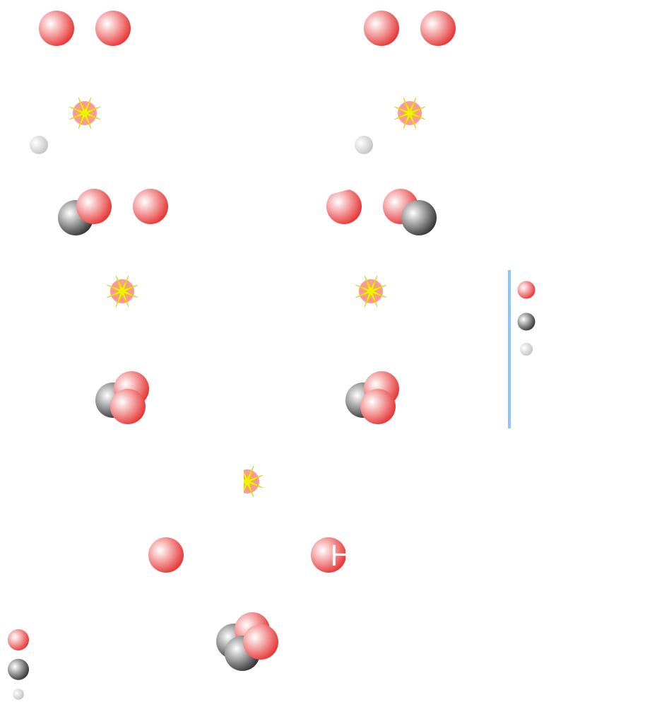
The pp chain is the main hydrogen-burning cycle in the present Sun.

First Step

The pp chain begins with

\[ p+p\to d+e^+ + \nu_e. \]

The emitted neutrino has a continuous spectrum with endpoint about

\[ E_\nu^{\max}\simeq 0.42~\mathrm{MeV}. \]

This is the largest solar-neutrino flux, but not the easiest component for water Cherenkov detectors.

pep Line

The related three-body reaction is

\[ p+e^-+p\to d+\nu_e. \]

It produces an almost monoenergetic neutrino:

\[ E_\nu \simeq 1.44~\mathrm{MeV}. \]

The pep flux is much smaller than pp, but the line is physically clean.

pp I Branch

After deuterium is produced,

\[ p+d\to {}^3\mathrm{He}+\gamma, \]

and the pp I branch ends through

\[ {}^3\mathrm{He}+{}^3\mathrm{He} \to {}^4\mathrm{He}+2p. \]

This branch produces pp neutrinos but no high-energy \(^8\mathrm{B}\) neutrinos.

pp II Branch

The chain can proceed through beryllium:

\[ {}^3\mathrm{He}+{}^4\mathrm{He}\to{}^7\mathrm{Be}+\gamma, \]

followed by electron capture:

\[ {}^7\mathrm{Be}+e^- \to {}^7\mathrm{Li}+\nu_e. \]

The main neutrino lines are approximately

\[ 0.862~\mathrm{MeV}, \qquad 0.384~\mathrm{MeV}. \]

pp III Branch

The high-energy branch is rare:

\[ {}^7\mathrm{Be}+p\to{}^8\mathrm{B}+\gamma, \]

then

\[ {}^8\mathrm{B}\to{}^8\mathrm{Be}^{*}+e^+ + \nu_e. \]

The \(^8\mathrm{B}\) flux is small, but its spectrum extends to high energy. This is why it is central for Super-Kamiokande-like measurements.

hep Tail

The rare reaction

\[ {}^3\mathrm{He}+p\to{}^4\mathrm{He}+e^+ + \nu_e \]

produces the highest-energy solar neutrinos.

The flux is tiny. The importance is not total rate, but the far high-energy tail.

CNO Cycle

Cycle Map

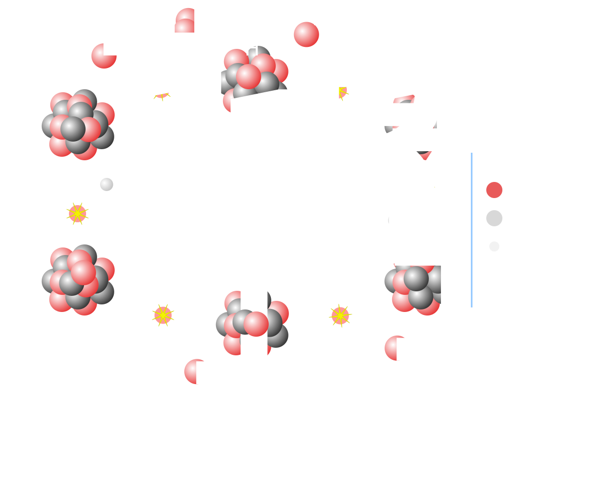
CNO catalytic loop and the smaller NO side branch.

CNO as a Catalyst Cycle

In the CNO cycle, carbon, nitrogen, and oxygen nuclei catalyze hydrogen burning.

The neutrino-producing beta decays are

\[ {}^{13}\mathrm{N}\to{}^{13}\mathrm{C}+e^+ + \nu_e, \]

\[ {}^{15}\mathrm{O}\to{}^{15}\mathrm{N}+e^+ + \nu_e, \]

\[ {}^{17}\mathrm{F}\to{}^{17}\mathrm{O}+e^+ + \nu_e. \]

Solar Model Inputs

Structure Equations

In Naumov’s notation, the stellar-structure equations are

\[ \frac{dM}{dR}=4\pi R^2\rho, \qquad \frac{dP}{dR}=-\frac{GM\rho}{R^2}, \]

\[ \frac{dL}{dR} = 4\pi R^2 \left[ \epsilon\rho -\rho\frac{d}{dt}\left(\frac{u}{\rho}\right) +\frac{P}{\rho}\frac{d\rho}{dt} \right], \qquad \frac{dT}{dR} = \nabla\frac{T}{P}\frac{dP}{dR}. \]

Here \(M(R)\) is the shell mass, \(L(R)\) is the energy flow through radius \(R\), \(u\) is the internal energy per unit volume, and

\[ \nabla=\frac{d\ln T}{d\ln P}. \]

Closure Equations

The four differential equations are not closed until the microphysics is specified:

\[ \rho=\rho(P,T,\{X_a\}), \qquad \kappa=\kappa(P,T,\{X_a\}), \qquad \epsilon=\epsilon(P,T,\{X_a\}). \]

They provide the equation of state, opacity, and nuclear energy-generation rate. The pressure is, in general,

\[ P=P_{\rm gas}+P_{\rm rad}+\frac{B^2}{8\pi}, \]

with the magnetic term usually neglected in standard solar models.

Transport Gradients

The temperature gradient is decomposed as

\[ \nabla = \nabla_{\rm rad} +\nabla_{\rm cond} +\nabla_{\rm conv}. \]

For radiative transfer in local thermodynamic equilibrium, in natural units,

\[ \nabla_{\rm rad} = \frac{3}{16\pi aG} \frac{\kappa P}{T^4} \frac{L}{M}. \]

Convection starts when the radiative gradient exceeds the adiabatic one:

\[ \nabla_{\rm rad}> \nabla_{\rm ad}, \qquad \nabla_{\rm ad} = \left(\frac{\partial\ln T}{\partial\ln P}\right)_s. \]

This is why opacity, composition, and the treatment of convection enter solar-neutrino predictions.

What Enters the Solar-Neutrino Calculation

For the masterclass we take as input:

• total fluxes \(\Phi_i\);
• spectral shapes \(f_i(E)\);
• radial production distributions;
• electron-density profile \(n_e(r)\);
• uncertainties or toy nuisance parameters.

We do not solve the solar model. We use its output.

Vacuum Oscillations

Time Evolution

• Prepare a neutrino as \(|\nu_e\rangle\) at \(t=0\):

\[ |\nu(0)\rangle = \cos\theta\,|\nu_1\rangle + \sin\theta\,|\nu_2\rangle. \]

• In vacuum each mass state evolves with its own phase:

\[ |\nu(t)\rangle = \cos\theta\,e^{-iE_1t}|\nu_1\rangle + \sin\theta\,e^{-iE_2t}|\nu_2\rangle. \]

Time Evolution

• The survival amplitude is

\[ A_{ee}(t) = \langle\nu_e|\nu(t)\rangle = \cos^2\theta\,e^{-iE_1t} + \sin^2\theta\,e^{-iE_2t}. \]

• The transition amplitude is

\[ A_{e\mu}(t) = \langle\nu_\mu|\nu(t)\rangle = \sin\theta\cos\theta \left(e^{-iE_2t}-e^{-iE_1t}\right). \]

Three Flavours

• In the full theory,

\[ |\nu_\alpha\rangle = \sum_{i=1}^3 U_{\alpha i}^{*}|\nu_i\rangle, \qquad \alpha=e,\mu,\tau. \]

• The PMNS matrix is described by three angles and one CP phase:

\[ U_{\rm PMNS} = R_{23}(\theta_{23})\, U_{13}(\theta_{13},\delta_{\rm CP})\, R_{12}(\theta_{12}). \]

• For solar neutrinos the dominant vacuum scale is \(\Delta m_{21}^2\) with angle \(\theta_{12}\); \(\theta_{13}\) gives a small but important correction:

\[ P_{ee}^{3\nu} \simeq \cos^4\theta_{13}\,P_{ee}^{2\nu} + \sin^4\theta_{13}. \]

3x3 Matrix

With \(c_{ij}\equiv\cos\theta_{ij}\) and \(s_{ij}\equiv\sin\theta_{ij}\),

\[ \small U_{\rm PMNS} = \begin{pmatrix} 1&0&0\\ 0&c_{23}&s_{23}\\ 0&-s_{23}&c_{23} \end{pmatrix} \begin{pmatrix} c_{13}&0&s_{13}e^{-i\delta_{\rm CP}}\\ 0&1&0\\ -s_{13}e^{i\delta_{\rm CP}}&0&c_{13} \end{pmatrix} \begin{pmatrix} c_{12}&s_{12}&0\\ -s_{12}&c_{12}&0\\ 0&0&1 \end{pmatrix}. \]

• Majorana phases are omitted; they do not affect oscillation probabilities.
• Solar neutrinos mainly probe \(\theta_{12}\) and \(\Delta m_{21}^2\), with a controlled \(\theta_{13}\) correction.

Flavor Change in Matter

Vacuum Matrix

Vacuum mixing in matrix form

\[ \nu_f= \begin{pmatrix} \nu_e\\ \nu_x \end{pmatrix}, \qquad \nu_f=U(\theta)\nu_m. \]

\[ U(\theta) = \begin{pmatrix} \cos\theta & \sin\theta\\ -\sin\theta & \cos\theta \end{pmatrix}. \]

Hamiltonian

\[ i\frac{d}{dt}\nu_f = H_{\rm vac}\nu_f, \qquad H_{\rm vac} = U \begin{pmatrix} \frac{m_1^2}{2E} & 0\\ 0 & \frac{m_2^2}{2E} \end{pmatrix} U^\dagger. \]

Vacuum Matrix

After subtracting an irrelevant trace

\[ H_{\rm vac} = \frac{\Delta m^2}{4E} \begin{pmatrix} -\cos2\theta & \sin2\theta\\ \sin2\theta & \cos2\theta \end{pmatrix}. \]

The Schroedinger equation

• Sum up vacuum and matter Hamiltonians: \[ i\frac{d}{dt}\begin{pmatrix} \nu_e\\ \nu_\mu \end{pmatrix} = \begin{pmatrix} -\frac{\Delta m^2}{4E}\cos2\theta +V_e(x) & \frac{\Delta m^2}{4E}\sin2\theta\\ \frac{\Delta m^2}{4E}\sin2\theta & \frac{\Delta m^2}{4E}\cos2\theta \end{pmatrix} \begin{pmatrix} \nu_e\\ \nu_\mu \end{pmatrix} \equiv H_f(x)\begin{pmatrix} \nu_e\\ \nu_\mu \end{pmatrix}. \]
• How to solve it?

Diagonalization

• Introduce a \(2\times 2\) matrix \(U(\theta_m)=\begin{pmatrix}\cos\theta_m& \sin\theta_m\\ -\sin\theta_m & \cos\theta_m\end{pmatrix}\) and a new matter states: \[ \nu_f = U(\theta_m)\,\nu_m. \]
• Multiply the Schroediner equation by \(U^\dagger(\theta_m)\) from the left and by \(U(\theta_m)\) from the right (assume \(n_e(x)=\mathrm{const}\)): \[ i\frac{d}{dt}\nu_m = U^\dagger(\theta_m) H_f(x)U(\theta_m)\nu_m \equiv H_m(x)\nu_m \]
• Choose \(U(\theta_m)\) to make \(H_m(x)\) diagonal.

Eigenstates

• Vacuum and matter states:

\[ |\nu_e\rangle = \cos\theta_m|\nu_1^m\rangle + \sin\theta_m|\nu_2^m\rangle. \]

• Vacuum and matter mixing angles:

\[ \tan2\theta_m = \frac{\Delta m^2\sin2\theta} {\Delta m^2\cos2\theta-2EV_e}. \]

• Vacuum and matter mass splittings:

\[ \Delta m_m^2 = \Delta m^2 \sqrt{ \left(\cos2\theta-\frac{2EV_e}{\Delta m^2}\right)^2 + \sin^2 2\theta }. \]

• After subtracting the trace, the eigenvalues are

\[ \lambda_\pm = \pm\frac{\Delta m_m^2}{4E}. \]

Probability

• In constant-density matter the vacuum formula survives with vacuum quantities replaced by matter quantities:

\[ P_{ee}^{\rm matter} = 1-\sin^2 2\theta_m\, \sin^2\!\left( \frac{\Delta m_m^2 L}{4E} \right). \]

• The appearance probability is

\[ P_{ex}^{\rm matter} = 1-P_{ee}^{\rm matter}. \]

• For varying density one evolves through layers, or uses adiabatic following when the density changes slowly.

Variable Density

• In the Sun the density changes with radius:

\[ H_f(R) = H_{\rm vac} + \begin{pmatrix} V_e(R)&0\\ 0&0 \end{pmatrix}. \]

• Define instantaneous matter eigenstates:

\[ H_f(R)|\nu_i^m(R)\rangle = \lambda_i(R)|\nu_i^m(R)\rangle. \]

• Adiabatic evolution means

\[ \left|\frac{d\theta_m}{dR}\right| \ll |\lambda_2-\lambda_1| = \frac{\Delta m_m^2(R)}{2E}. \]

PEANUTS Daytime Table

The masterclass table

oscillation_probabilities_grid.csv

stores the PEANUTS daytime result for \(^8\mathrm{B}\) neutrinos:

\[ P_{ee}^{day} = P_{ee}^{day} \left(E_\nu;\sin^2\theta_{12},\Delta m^2_{21}\right). \]

PEANUTS computes this from the solar model, the \(^8\mathrm{B}\) production profile, and adiabatic solar propagation.

Earth Matter

Day and Night

During the day, solar neutrinos reach the detector without crossing the Earth.

At night they can propagate through Earth matter before detection.

This modifies the mass-state mixture projected onto \(\nu_e\):

\[ P_{ee}^{\mathrm{night}}(E,\eta) \ne P_{ee}^{\mathrm{day}}(E). \]

\(\eta\) denotes the nadir angle.

Regeneration

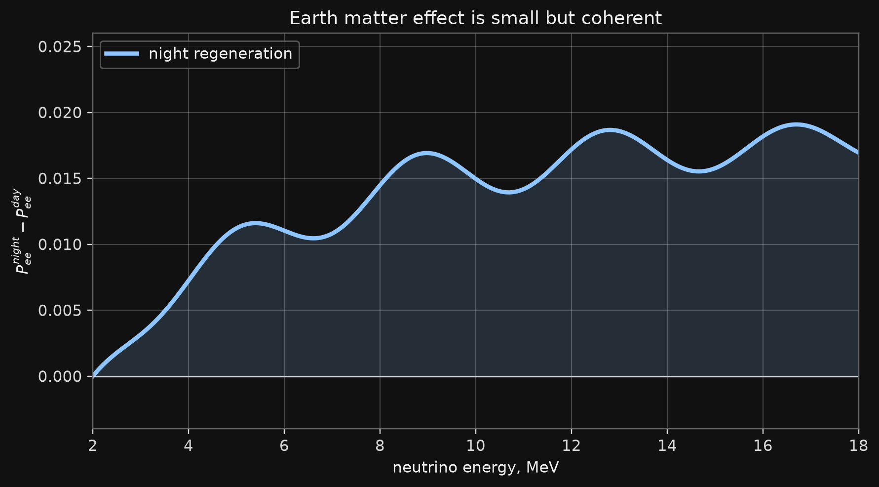
The Earth matter correction is usually small:

\[ \Delta P_{ee}^{\oplus} = P_{ee}^{\mathrm{night}}-P_{ee}^{\mathrm{day}}. \]

It is nevertheless coherent and measurable statistically in large detectors.

The optional masterclass table

earth_regeneration_grid.csv

stores this quantity computed with PEANUTS Earth propagation for several nadir angles \(\eta\).

Regeneration

The table

earth_regeneration_parameter_scan.csv

uses the same PEANUTS calculation at selected \(E_\nu\) and \(\eta\) values while scanning \((\sin^2\theta_{12},\Delta m^2_{21})\).

Day-Night Asymmetry

A common observable is

\[ A_{\mathrm{DN}} = 2\frac{N_{\mathrm{night}}-N_{\mathrm{day}}} {N_{\mathrm{night}}+N_{\mathrm{day}}}. \]

Detection

Elastic Scattering Cross Section

For neutrino-electron scattering, neglecting radiative corrections, the differential cross section has the structure

\[ \frac{d\sigma}{dT} = \frac{2G_F^2m_e}{\pi} \left[ g_L^2 +g_R^2\left(1-\frac{T}{E_\nu}\right)^2 -g_Lg_R\frac{m_eT}{E_\nu^2} \right]. \]

The coupling constants differ between \(\nu_e e\) and \(\nu_{\mu,\tau}e\) scattering.

Weak Couplings

Using \(s_W^2=\sin^2\theta_W\simeq0.231\):

channel	\(g_L\)	value	\(g_R\)	value
\(\nu_e e\to\nu_e e\)	\(\frac{1}{2}+s_W^2\)	\(0.731\)	\(s_W^2\)	\(0.231\)
\(\nu_{\mu,\tau}e\to\nu_{\mu,\tau}e\)	\(-\frac{1}{2}+s_W^2\)	\(-0.269\)	\(s_W^2\)	\(0.231\)

For antineutrinos the roles of \(g_L\) and \(g_R\) are interchanged in the recoil-energy dependence.

Approximate Total Cross Sections

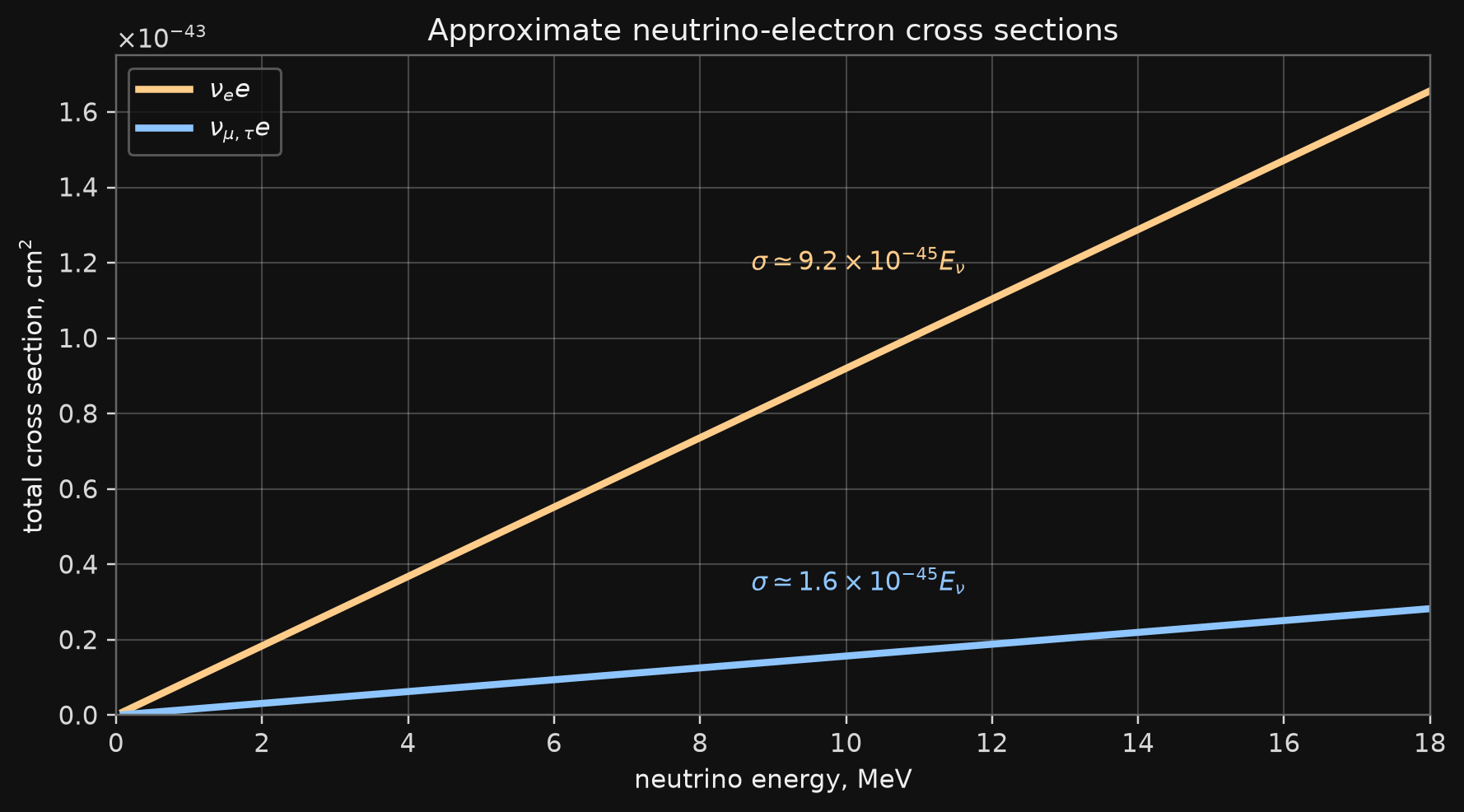
Linear high-energy approximations in cm\(^2\) for solar-neutrino energies. The full recoil spectrum is used only in precision analyses.

Statistical Inference

Pseudoexperiment

For binned expected counts \(\mu_i\),

\[ n_i \sim \mathrm{Poisson}(\mu_i). \]

A fixed random seed gives a reproducible pseudoexperiment for all students.

The point is to separate the true model from one possible observed dataset.

Poisson Chi-Square

For counting data use

\[ \chi^2 = 2\sum_i \left[ \mu_i-n_i+n_i\ln\frac{n_i}{\mu_i} \right]. \]

For \(n_i=0\), the logarithmic term is defined as zero.