Oscillations in Vacuum. Three Flavors and the PMNS Matrix

Introduction to Neutrino Physics

Dmitry V. Naumov

JINR

Three Flavors

Two Bases

The charged lepton at production or detection determines the flavor:

\[ \nu_e,\qquad\nu_\mu,\qquad\nu_\tau. \]

These are three states distinguishable by the weak interaction.

In vacuum, three eigenstates propagate:

\[ H_0|\nu_i\rangle=E_i|\nu_i\rangle, \qquad i=1,2,3. \]

Each acquires a phase \(e^{-i(E_it-p_iL)}\). Of the three phase differences, two are independent.

The three angles describe the relative orientation of the bases; the complex phase appears in the interference of the three mass waves.

Mixing Matrix

\[ U=\begin{pmatrix} U_{e1}&U_{e2}&U_{e3}\\ U_{\mu1}&U_{\mu2}&U_{\mu3}\\ U_{\tau1}&U_{\tau2}&U_{\tau3} \end{pmatrix}, \qquad \boxed{|\nu_\alpha\rangle =\sum_{i=1}^{3}U_{\alpha i}^*|\nu_i\rangle}. \]

  • Row \(\alpha\) corresponds to the flavor; column \(i\) corresponds to the mass state.
  • The number \(|U_{\alpha i}|^2\) shows the fraction of the mass component \(i\) in the flavor state \(\alpha\).
  • The transition from one basis to the other preserves norms and scalar products.

Ones on the Diagonal, Zeros Off It

Unitarity means

\[ \boxed{UU^\dagger=U^\dagger U= \begin{pmatrix} 1&0&0\\ 0&1&0\\ 0&0&1 \end{pmatrix}}. \]

Rows:

\[ \sum_i|U_{\alpha i}|^2=1, \qquad \sum_iU_{\alpha i}U_{\beta i}^*=0 \quad(\alpha\ne\beta). \]

Columns:

\[ \sum_\alpha|U_{\alpha i}|^2=1, \qquad \sum_\alpha U_{\alpha i}^*U_{\alpha j}=0 \quad(i\ne j). \]

The normalizations give three ones on the diagonal. The six off-diagonal zeros are pairwise conjugate: these are three complex, that is, six real conditions. In total, \(U^\dagger U=I\) amounts to \(3+6=9\) real conditions; for a square matrix, \(UU^\dagger=I\) follows from this and adds no new conditions.

What an Experimental Test Means

  • If \(U\) is written as a product of three unitary rotations, the equality \(U^\dagger U=I\) holds for any values of the angles and the phase.
  • An experimental test requires determining the elements through different channels of production, disappearance, and appearance, allowing the data to violate the normalization and orthogonality conditions.
  • The normalizations also require information on the absolute rates of weak processes, fluxes, and cross sections; the shapes of the curves in \(L/E\) alone are not enough.

A good agreement of the fit with a unitary matrix tests the model as a whole. Testing unitarity itself requires an analysis in which its constraints are not imposed in advance.

Three Angles and One Phase

Three Rotations and One Phase

Let \(c_{ij}=\cos\theta_{ij}\), \(s_{ij}=\sin\theta_{ij}\), and \(\delta\equiv\delta_{\rm CP}\). The standard convention has the form

\[ \boxed{U=R_{23}U_{13}(\delta_{\rm CP})R_{12}}, \]

\[ \begin{aligned} R_{23}&=\begin{pmatrix}1&0&0\\0&c_{23}&s_{23}\\0&-s_{23}&c_{23}\end{pmatrix}, &U_{13}&=\begin{pmatrix}c_{13}&0&s_{13}e^{-i\delta}\\0&1&0\\-s_{13}e^{i\delta}&0&c_{13}\end{pmatrix}, &R_{12}&=\begin{pmatrix}c_{12}&s_{12}&0\\-s_{12}&c_{12}&0\\0&0&1\end{pmatrix}. \end{aligned} \]

From right to left: \(R_{12}\) rotates in the \(12\) plane, \(U_{13}\) acts in the \(13\) plane and carries the phase, \(R_{23}\) rotates in the \(23\) plane. Each factor is unitary.

PMNS Matrix

Multiplying the three factors, we obtain

\[ \boxed{ U=\begin{pmatrix} c_{12}c_{13}&s_{12}c_{13}&s_{13}e^{-i\delta}\\ -s_{12}c_{23}-c_{12}s_{23}s_{13}e^{i\delta} &c_{12}c_{23}-s_{12}s_{23}s_{13}e^{i\delta} &s_{23}c_{13}\\ s_{12}s_{23}-c_{12}c_{23}s_{13}e^{i\delta} &-c_{12}s_{23}-s_{12}c_{23}s_{13}e^{i\delta} &c_{23}c_{13} \end{pmatrix}}. \]

The first row and the third column can be read off immediately:

\[ \frac{|U_{e2}|}{|U_{e1}|}=\tan\theta_{12},\qquad |U_{e3}|^2=\sin^2\theta_{13},\qquad \frac{|U_{\mu3}|}{|U_{\tau3}|}=\tan\theta_{23}. \]

The multiplication and additional checks are in the exercises for the lecture.

What Is Visible in the Flavor Fractions

  • \(\theta_{12}\) distributes the electron row between columns \(1\) and \(2\).
  • \(\theta_{13}\) determines the small electron fraction in column \(3\): \(|U_{e3}|^2=0.022\) (narrow light-blue strip).
  • \(\theta_{23}\) divides column \(3\) between \(\mu\) and \(\tau\).
  • \(\delta_{\rm CP}\) through \(\cos\delta_{\rm CP}\) changes the fractions of \(\mu\) and \(\tau\) in columns \(1\) and \(2\).

The example is computed from the NuFIT 6.1 best-fit point (NO, IC24 + SK-atm); the fractions of each column sum to one up to rounding.

Dirac and Majorana: How Many Phases?

A unitary matrix \(U\) of size \(3\times3\) contains three angles and six phases.

  • In the mass basis:

\[ \begin{aligned} \mathcal L_{\rm CC} &=-\frac{g}{\sqrt2}\,W^-_\mu \sum_{\alpha,i}\bar\ell_{\alpha L}\gamma^\mu U_{\alpha i}\nu_{iL} +\mathrm{h.c.},\\ \mathcal L_{\rm mass} &=-\sum_\alpha m_\alpha\bar\ell_\alpha\ell_\alpha -\sum_i m_i\bar\nu_i\nu_i. \end{aligned} \]

  • The mass terms are preserved under a change of field phases:

\[ \ell_\alpha\mapsto e^{i\phi_\alpha}\ell_\alpha, \qquad \nu_i\mapsto e^{i\psi_i}\nu_i. \]

  • The charged current keeps its form if

\[ \boxed{U_{\alpha i}'= e^{i(\phi_\alpha-\psi_i)}U_{\alpha i}}. \]

  • On \(U\), the differences \(\phi_\alpha-\psi_i\) act. A common shift of all six phases:

\[ \begin{gathered} \phi_\alpha\mapsto\phi_\alpha+\chi,\quad \psi_i\mapsto\psi_i+\chi:\\ (\phi_\alpha+\chi)-(\psi_i+\chi)=\phi_\alpha-\psi_i. \end{gathered} \]

  • This shift does not change \(U\). Subtracting \(\psi_3\) from all phases, we obtain five independent parameters:

\[ \phi_e-\psi_3,\ \ \phi_\mu-\psi_3,\ \ \phi_\tau-\psi_3,\ \ \psi_1-\psi_3,\ \ \psi_2-\psi_3. \]

  • Five independent rephasings remove five of the six phases \(U\): \(\boxed{6-5=1}\). The physical phase \(\delta_{\rm CP}\) remains.

The masses \(m_i\) are chosen real and positive. \(\widetilde U\) denotes the full mixing matrix.

  • Majorana mass:

\[ \mathcal L_{\rm mass}^{(M)} =-\frac12\sum_i m_i\,\overline{\nu_{iL}^{\,c}}\nu_{iL} +\mathrm{h.c.} \]

  • For \(\nu_{iL}\mapsto e^{i\psi_i}\nu_{iL}\):

\[ \overline{\nu_{iL}^{\,c}}\nu_{iL} \mapsto e^{2i\psi_i}\overline{\nu_{iL}^{\,c}}\nu_{iL}. \]

For fixed \(m_i\), only \(\psi_i=0,\pi\) are allowed.

  • Three rephasings of the charged leptons remove the three common row phases. What remain are \(\boxed{6-3=3}\) physical phases: \(\delta_{\rm CP}\) and two Majorana phases.
  • The charged leptons remain Dirac. Their mass terms \(-m_\alpha\bar\ell_\alpha\ell_\alpha\) are preserved under \(\ell_\alpha\mapsto e^{i\phi_\alpha}\ell_\alpha\).

\[ \widetilde U'=D_\ell\widetilde U,\qquad D_\ell=\operatorname{diag}(e^{i\phi_e},e^{i\phi_\mu},e^{i\phi_\tau}). \]

  • Multiplication from the left changes the whole row \(\alpha\):

\[ \widetilde U_{\alpha i}'=e^{i\phi_\alpha}\widetilde U_{\alpha i} \qquad\text{for all }i. \]

A single \(\phi_\alpha\) multiplies the entire row \(\alpha\) by a common factor. The relative phases of its elements are preserved.

After the phases of the charged leptons are chosen, the full matrix can be written as \(\widetilde U=U(\delta)D_M\). In \(U(\delta)\) there are three angles and one phase \(\delta_{\rm CP}\).

  • The factor \(e^{i\eta_i}\) belongs to the mass state \(\nu_i\), that is, to column \(i\):

\[ \widetilde U_{\alpha i}=U_{\alpha i}(\delta)e^{i\eta_i}. \]

This is how multiplication from the right by

\[ D_M=\operatorname{diag}(e^{i\eta_1},e^{i\eta_2},e^{i\eta_3}). \]

acts.

  • In \(D_M\) with three \(\eta_i\), one common phase is redundant. The factor \(e^{i\eta_1}\) on the whole matrix is removed by the uniform replacement \(\ell_\alpha\mapsto e^{-i\eta_1}\ell_\alpha\), which is already included in the three row rephasings. Physically, the differences \(\eta_2-\eta_1\) and \(\eta_3-\eta_1\) remain.
  • Majorana phases \(\alpha_{j1}=2(\eta_j-\eta_1)\):

\[ D_M=\operatorname{diag} \left(1,e^{i\alpha_{21}/2},e^{i\alpha_{31}/2}\right). \]

  • In oscillations, the column phase cancels:

\[ \widetilde U_{\beta i}\widetilde U_{\alpha i}^{*} =U_{\beta i}U_{\alpha i}^{*}e^{i\eta_i}e^{-i\eta_i} =U_{\beta i}U_{\alpha i}^{*}. \]

  • In \(0\nu\beta\beta\), the phases double:

\[ m_{\beta\beta}=\left|\sum_i m_i\widetilde U_{ei}^{2}\right|, \qquad \widetilde U_{ei}^{2}=U_{ei}^{2}e^{2i\eta_i}. \]

Paul Dirac and Ettore Majorana

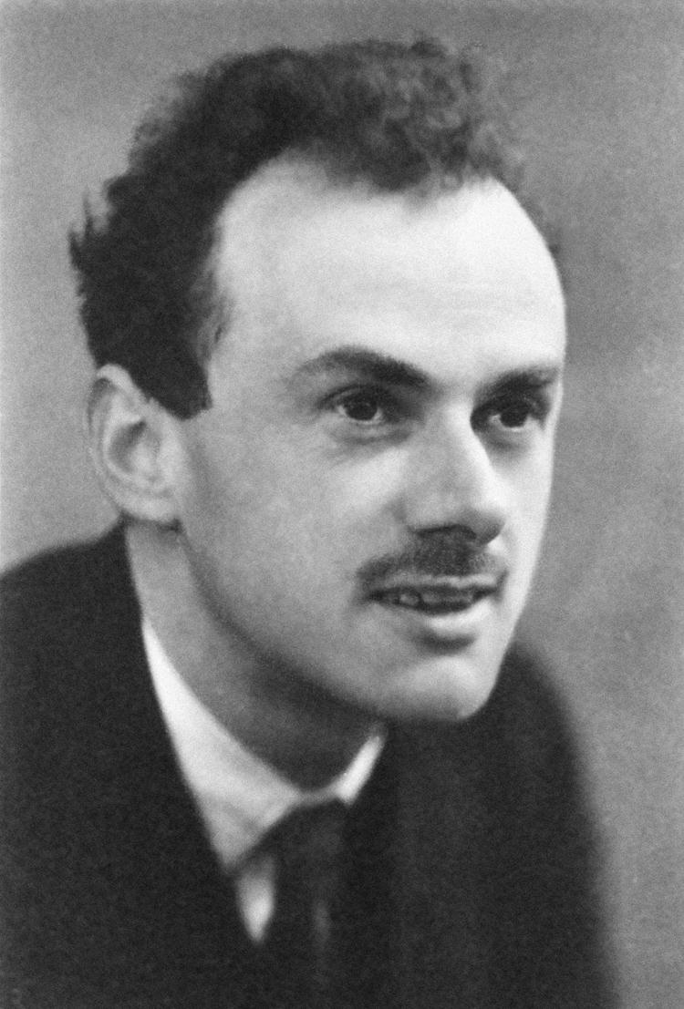
Paul Dirac

1902–1984. The relativistic Dirac equation described a fermion with spin \(1/2\) and led to the prediction of the electron’s antiparticle. In 1933, Dirac shared the Nobel Prize in Physics with Erwin Schrödinger.
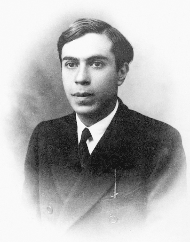
Ettore Majorana

1906 — disappeared in 1938. In 1937, Majorana constructed a theory of a neutral fermion that coincides with its own antiparticle. Whether this description applies to the neutrino is for experiment to say.

From State to Probability

Transition Amplitude

The source prepares the flavor \(\alpha\):

\[ |\nu_\alpha;0\rangle=\sum_iU_{\alpha i}^*|\nu_i\rangle. \]

Each mass component propagates with its own phase.

For an ultrarelativistic neutrino after a distance \(L\):

\[ |\nu_\alpha;L\rangle =\sum_iU_{\alpha i}^* \exp\!\left(-i\frac{m_i^2L}{2E}\right)|\nu_i\rangle. \]

The phase common to the three components is dropped: it does not enter the probability.

The detector projects the state onto the flavor \(\beta\). The orthogonality of the mass states leaves a single sum:

\[ \boxed{ \mathcal A_{\alpha\to\beta}(L,E) =\sum_{i=1}^{3} U_{\beta i}U_{\alpha i}^* e^{-im_i^2L/(2E)} }. \]

In each term one can see the production, propagation, and detection of a single mass component.

Three Pairs, Two Independent Differences

Denote

\[ \Delta_{ij}=\frac{\Delta m_{ij}^2L}{4E}, \qquad \Delta m_{ij}^2=m_i^2-m_j^2. \]

Of the three possible pairs \(21\), \(31\) and \(32\), two are independent:

\[ \boxed{\Delta m_{31}^2=\Delta m_{32}^2+\Delta m_{21}^2}. \]

  • The fast oscillations are set by the atmospheric splitting \(|\Delta m_{31}^2|\approx|\Delta m_{32}^2|\).
  • The slow modulation is set by the solar one, \(\Delta m_{21}^2\).
  • The sign of the large splitting sets the mass ordering. To extract it from the data, one compares the energy dependences, including those in matter.

Squared Amplitude

Put

\[ a_i=U_{\beta i}U_{\alpha i}^*e^{-im_i^2L/(2E)}, \qquad \mathcal A_{\alpha\to\beta}=a_1+a_2+a_3. \]

Then the probability is a sum of three diagonal contributions and the interference of the three pairs:

\[ \boxed{ P_{\alpha\to\beta}=\left|\sum_i a_i\right|^2 =\sum_i|a_i|^2+2\sum_{i>j}\operatorname{Re}(a_i a_j^*) }. \]

For a compact notation we introduce

\[ X_{\alpha\beta}^{ij} =U_{\alpha i}^*U_{\beta i}U_{\alpha j}U_{\beta j}^*. \]

The real part of \(X^{ij}\) gives the familiar oscillation maxima. The imaginary part will be needed when comparing neutrinos and antineutrinos. The full expansion of the sum is exercise 10.3.

Survival and Appearance

For \(\beta=\alpha\) all the products \(X_{\alpha\alpha}^{ij}\) are real:

\[ \boxed{ P_{\alpha\to\alpha} =1-4\sum_{i>j}|U_{\alpha i}|^2|U_{\alpha j}|^2 \sin^2\Delta_{ij} }. \]

  • The deficit of flavor \(\alpha\) measures the moduli of row \(\alpha\) and the periods set by \(\Delta m_{ij}^2\). In vacuum the formula is the same for neutrinos and antineutrinos.

For \(\alpha\ne\beta\):

\[ \boxed{ P_{\alpha\to\beta} =-4\sum_{i>j}\operatorname{Re}X_{\alpha\beta}^{ij} \sin^2\Delta_{ij} +2\sum_{i>j}\operatorname{Im}X_{\alpha\beta}^{ij} \sin2\Delta_{ij} }. \]

  • Here products of elements from two rows enter, so the appearance channel is sensitive also to their relative phases. The interference part depends on \(\delta_{\rm CP}\).

The sum of the three final probabilities for a fixed initial flavor equals one. The direct derivation and the two-flavor limit are in exercise 10.3.

Neutrinos and Antineutrinos in Vacuum

For antineutrinos the mixing matrix is complex conjugated:

\[ \boxed{\bar U=U^*}. \]

Under this replacement

\[ \operatorname{Re}X^{ij}\longrightarrow\operatorname{Re}X^{ij}, \qquad \operatorname{Im}X^{ij}\longrightarrow-\operatorname{Im}X^{ij}. \]

Consequently, in the appearance channel the difference equals

\[ \boxed{ A_{\alpha\beta}^{\rm CP} =P(\nu_\alpha\to\nu_\beta) -P(\bar\nu_\alpha\to\bar\nu_\beta) =4\sum_{i>j}\operatorname{Im}X_{\alpha\beta}^{ij} \sin2\Delta_{ij} }. \]

For the survival channel in vacuum \(A_{\alpha\alpha}^{\rm CP}=0\).

Probabilities as Functions of Energy and Length

Three Probabilities in One Figure

Initial flavor
Particle
Mass ordering
\(L/E\) 9900 \(\mathrm{km/GeV}\)
\(P_{\alpha\to e}=1\) \(P_{\alpha\to\mu}=1\) \(P_{\alpha\to\tau}=1\)
\(P_{\alpha\to e}\)
0.000
\(P_{\alpha\to\mu}\)
1.000
\(P_{\alpha\to\tau}\)
0.000
\(\sum_{\beta=e,\mu,\tau}P_{\alpha\to\beta}=\) 1.000

The point shows \((P_{\alpha\to e},P_{\alpha\to\mu},P_{\alpha\to\tau})\). The path \(x=L/L_{\rm osc}^{21}\) is extended to three solar periods. The NO and IO buttons set the angles and phase of the best-fit point of the corresponding ordering: NuFIT 6.1, IC24 + SK-atm.

CP Violation

Comparing Conjugate Channels

In vacuum one compares transitions at the same \(L\) and \(E\):

\[ \nu_\alpha\to\nu_\beta, \qquad \bar\nu_\alpha\to\bar\nu_\beta. \]

  • For two flavors the mixing matrix can be made real.

  • The three-flavor matrix admits a physical complex phase, which can give a nonzero probability difference.

  • In long-baseline accelerator experiments, Earth’s matter also affects this comparison.

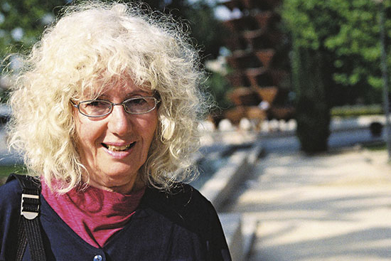
Cecilia Jarlskog

In 1985 Jarlskog proposed, for quarks, a quantity that does not change under redefinition of the field phases:

\[ \boxed{ J_{\rm CP} =\operatorname{Im} \left(U_{e2}^*U_{\mu2}U_{e1}U_{\mu1}^*\right) }. \]

In the standard parametrization

\[ \boxed{ J_{\rm CP} =c_{12}s_{12}c_{23}s_{23}c_{13}^2s_{13}\sin\delta_{\rm CP} }. \]

\(J_{\rm CP}\ne0\) only if all three angles differ from \(0\) and \(90^\circ\), and \(\sin\delta_{\rm CP}\ne0\).

Reminder

Rephasing the fields \(\ell_\alpha\to e^{i\varphi_\alpha}\ell_\alpha\), \(\nu_i\to e^{i\psi_i}\nu_i\) does not change the physics (the “Dirac particle” tab).

  • The field phases are arbitrary: \(U_{\alpha i}\to e^{i(\varphi_\alpha-\psi_i)}U_{\alpha i}\).
  • A single element changes its phase, so its phase is unobservable.
  • Of two elements only the pair \(U_{\alpha i}U_{\alpha i}^*=|U_{\alpha i}|^2\) is invariant, and it is real.
  • Rows \(\alpha\ne\beta\) and columns \(i\ne j\) give the quadruple

\[ Q_{\alpha\beta}^{ij}=U_{\alpha i}U_{\beta j}U_{\alpha j}^*U_{\beta i}^*. \]

  • Each index enters once in \(U\) and once in \(U^*\): the phases cancel, while \(Q\) can be complex.
  • For antineutrinos \(U\to U^*\), therefore \(\operatorname{Im}Q\to-\operatorname{Im}Q\): this is a CP-odd quantity.

Levi-Civita symbol

\(\varepsilon_{e\mu\tau}=\varepsilon_{123}=1\).

Swapping two indices changes the sign; if two indices coincide, \(\varepsilon=0\).

  • The pair of rows \(\{\alpha,\beta\}\) can be chosen in three ways, the pair of columns \(\{i,j\}\) also in three.
  • This gives \(3\cdot3=9\) submatrices \(2\times2\) and nine quadruples \(Q\).

Statement. For three flavors their imaginary parts coincide up to sign:

\[ \boxed{ \operatorname{Im}Q_{\alpha\beta}^{ij} =J_{\rm CP}\sum_{\gamma,k}\varepsilon_{\alpha\beta\gamma}\,\varepsilon_{ijk} }, \qquad J_{\rm CP}=\operatorname{Im}Q_{e\mu}^{12}. \]

  • The sign is set by the product \(\varepsilon_{\alpha\beta\gamma}\varepsilon_{ijk}\).
  • Hence, for three flavors there is one CP-odd mixing invariant.

What is needed

Orthogonality of rows: \(\sum_iU_{\alpha i}U_{\beta i}^*=0\) for \(\alpha\ne\beta\).

\(\operatorname{Im}|z|^2=0\), \(\operatorname{Im}(w z^*)=-\operatorname{Im}(z w^*)\).

  1. For rows \(\alpha\ne\beta\) put \(z_i=U_{\alpha i}U_{\beta i}^*\). Orthogonality: \(z_1+z_2+z_3=0\).
  2. The product of two terms gives the quadruple: \(z_1z_2^*=Q_{\alpha\beta}^{12}\).
  3. Substitute \(z_3=-(z_1+z_2)\):

\[ z_2z_3^*=-z_2z_1^*-|z_2|^2 \;\Rightarrow\; \operatorname{Im}(z_2z_3^*)=\operatorname{Im}(z_1z_2^*). \]

  1. Likewise \(\operatorname{Im}(z_3z_1^*)=\operatorname{Im}(z_1z_2^*)\), and swapping the columns changes the sign.
  2. Orthogonality of the columns repeats steps 1–4 for pairs of rows. \(\square\)
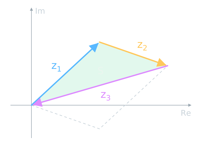
The vectors z1, z2, z3 close the unitarity triangle; the dashed line completes the parallelogram on z1 and z2

  • \(z_1+z_2+z_3=0\): the three vectors close a unitarity triangle.
  • The triangle is half of the parallelogram on \(z_1\) and \(z_2\):

\[ \boxed{ S=\frac12\left|z_1\times z_2\right| =\frac12\left|\operatorname{Im}(z_1^*z_2)\right| =\frac12|J_{\rm CP}| }. \]

  • All six triangles have the same area: three from rows and three from columns.
  • \(J_{\rm CP}=0\): the triangle degenerates into a segment.

Reminder

\(X_{\alpha\beta}^{ij}=U_{\alpha i}^*U_{\beta i}U_{\alpha j}U_{\beta j}^*\) enters the probability with \(\sin2\Delta_{ij}\) (slide “Squared Amplitude”).

  • Two flavors: \(z_1+z_2=0\), the triangle is degenerate, CP is conserved.
  • Oscillations: \(X^{ij}_{\alpha\beta}\) is also a quadruple, \(\operatorname{Im}X^{ij}_{\alpha\beta}=\pm J_{\rm CP}\). Therefore \(P(\nu_\alpha\to\nu_\beta)-P(\bar\nu_\alpha\to\bar\nu_\beta)\propto J_{\rm CP}\) (next slide).
  • Three distinct masses are needed: for \(\Delta m^2_{ij}=0\) the difference vanishes.
  • Survival: \(\varepsilon_{\alpha\alpha\gamma}=0\), no asymmetry.
  • Majorana phases of the columns cancel in each quadruple.
  • \(N\) flavors: \((N-1)(N-2)/2\) Dirac phases; for \(N\ge4\) a single \(J_{\rm CP}\) is not enough.

Jarlskog, 1985

For quarks

\[ \det[H_u,H_d]\propto iJ\,D_uD_d, \]

where \(H=MM^\dagger\), and \(D_q\) is the product of the squared-mass differences. Both the phase and the nondegenerate masses are needed.

\[ J_{\rm CP}=\frac18\sin2\theta_{12}\sin2\theta_{23} \sin2\theta_{13}\cos\theta_{13}\sin\delta_{\rm CP}. \]

  • Maximum: \(\theta_{12}=\theta_{23}=45^\circ\), \(|\sin\delta_{\rm CP}|=1\), and \(c_{13}^2s_{13}=(1-x)\sqrt x\) is maximal at \(x=\sin^2\theta_{13}=1/3\):

\[ |J_{\rm CP}|\le\frac1{6\sqrt3}\approx0.096,\qquad |U_{\alpha i}|^2=\frac13. \]

  • Leptons (NuFIT 6.1): \(J_{\rm CP}\approx0.034\sin\delta_{\rm CP}\); at the NO best-fit point \(J_{\rm CP}\approx-0.018\).
  • Quarks: \(J\approx3\cdot10^{-5}\).

Vacuum CP Asymmetry

For the channel \(e\to\mu\) the imaginary parts of the three interference products are expressed through a single \(J_{\rm CP}\). We obtain

\[ \boxed{ A_{e\mu}^{\rm CP} =16J_{\rm CP} \sin\Delta_{21}\sin\Delta_{32}\sin\Delta_{31} }. \]

  • If \(\theta_{13}=0\), then \(J_{\rm CP}\) also vanishes.
  • The factor \(\sin\Delta_{21}\): without the solar scale there is no CP effect in a long-baseline experiment.
  • By CPT \(P(\nu_\mu\to\nu_e)=P(\bar\nu_e\to\bar\nu_\mu)\), therefore \(A_{\mu e}^{\rm CP}=-A_{e\mu}^{\rm CP}\).

The derivation of the identity and an estimate of the size of the effect are homework exercise 10.4.

Mixing Matrix

Doing the Fit by Hand

We use three experimental results:

  • solar neutrinos: \(P_{ee}\simeq1/3\);
  • atmospheric and accelerator neutrinos: \(\sin^22\theta_{23}\simeq1\);
  • a small electron admixture of the third state: first put \(|U_{e3}|^2=0\).

We will need the normalizations of rows and columns, then orthogonality. The connection of the solar result with \(|U_{e2}|^2\) relies on the adiabatic matter effect; its physics will be derived in lecture 13.

Building the matrix step by step

Step 0 of 10

We start with an empty matrix

The rows correspond to the flavors of production and detection; the columns, to the mass states. We begin with the measurable fractions \(|U_{\alpha i}|^2\).

For now we leave \(|U_{e3}|^2=0\). This reveals the framework of the problem; the reactor result will be included at the end.

\(\bigl|U_{\alpha i}\bigr|^2\)
\(\nu_1\) \(\nu_2\) \(\nu_3\)
\(e\) \(\tfrac23\)\(\sqrt{\tfrac23}\)\(\pm\sqrt{\tfrac23}\)\(+\sqrt{\tfrac23}\)\(0.676\) \(\tfrac13\)\(\sqrt{\tfrac13}\)\(+\sqrt{\tfrac13}\)\(+\sqrt{\tfrac13}\)\(0.302\) \(0\)\(0\)\(0\)\(0\)\(0.022\)
\(\mu\) \(\tfrac16\)\(\sqrt{\tfrac16}\)\(\pm\sqrt{\tfrac16}\)\(-\sqrt{\tfrac16}\)\(0.112\) \(\tfrac13\)\(\sqrt{\tfrac13}\)\(+\sqrt{\tfrac13}\)\(+\sqrt{\tfrac13}\)\(0.428\) \(\tfrac12\)\(\sqrt{\tfrac12}\)\(+\sqrt{\tfrac12}\)\(+\sqrt{\tfrac12}\)\(0.459\)
\(\tau\) \(\tfrac16\)\(\sqrt{\tfrac16}\)\(\pm\sqrt{\tfrac16}\)\(+\sqrt{\tfrac16}\)\(0.212\) \(\tfrac13\)\(\sqrt{\tfrac13}\)\(-\sqrt{\tfrac13}\)\(-\sqrt{\tfrac13}\)\(0.270\) \(\tfrac12\)\(\sqrt{\tfrac12}\)\(+\sqrt{\tfrac12}\)\(+\sqrt{\tfrac12}\)\(0.518\)
The first ten steps: \(U_{e3}=0\). The last step: NuFIT 6.1, NO, IC24 + SK-atm (2025).

What this reconstruction gave

At zeroth order we obtain the matrix of squared moduli

\[ \boxed{ |U_0|^2= \begin{pmatrix} 2/3&1/3&0\\ 1/6&1/3&1/2\\ 1/6&1/3&1/2 \end{pmatrix}}. \]

  • Unitarity made it possible to fill in the entries that these experiments do not measure directly.
  • To fix the signs, one real unitary representative was constructed \(U_0\). Its phase \(\delta_{\rm CP}\) at \(U_{e3}=0\) is not observable.
  • Reactor data give \(|U_{e3}|^2\simeq0.0225\). The full matrix requires additional measurements and allows a complex phase.

The combined analysis of different sources reconstructed the whole matrix, but its unitarity was an initial condition of the reconstruction. For an independent test, one allows deviations from unitarity and cross-checks different channels.

What has been measured today

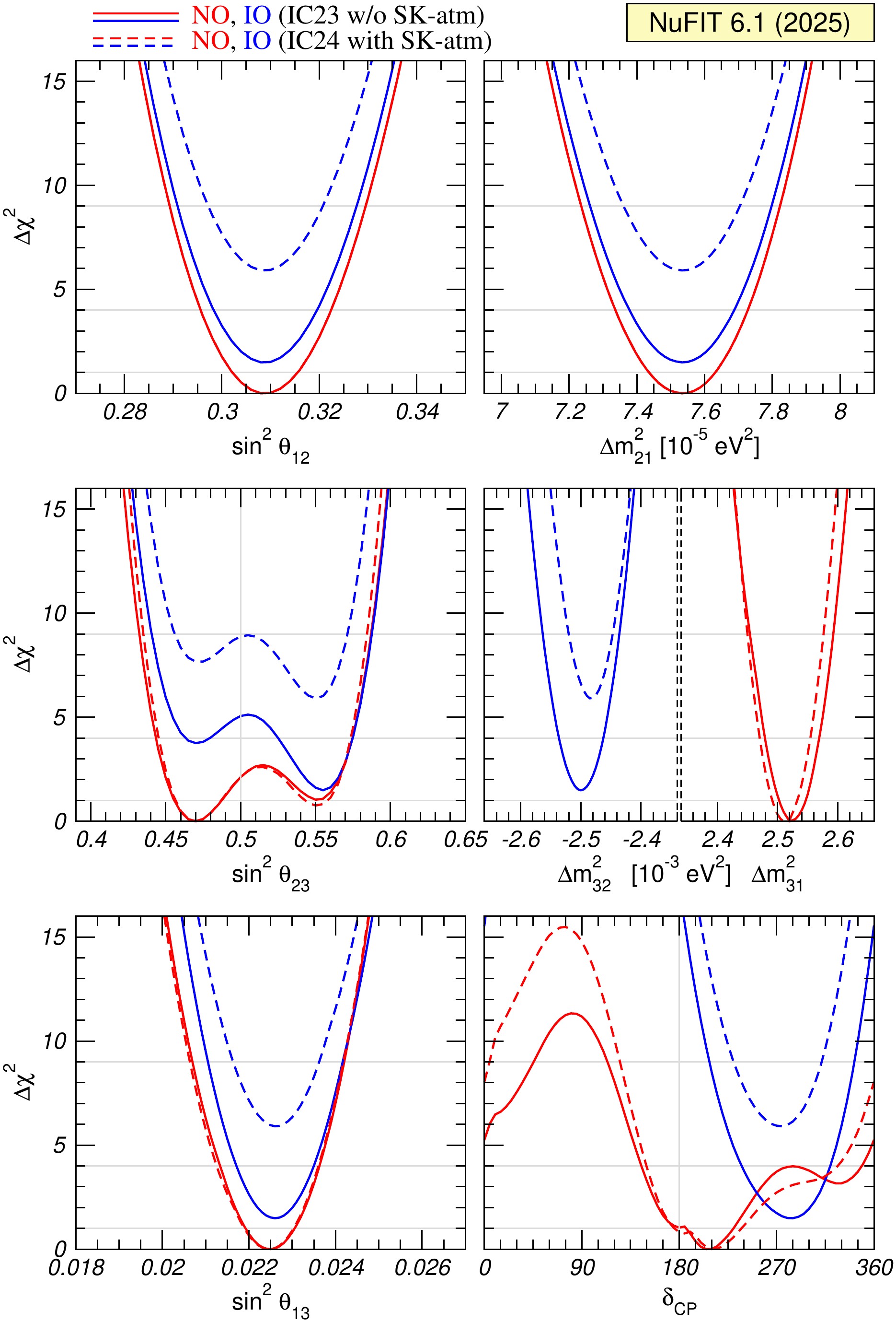
NuFIT 6.1: three angles

Normal mass ordering, atmospheric data IC24 and Super-Kamiokande. Best-fit values and \(3\sigma\) intervals:

Parameter Best-fit value \(3\sigma\) interval
\(\sin^2\theta_{12}\) \(0.3088\) \(0.2893\)–\(0.3295\)
\(\sin^2\theta_{13}\) \(0.02248\) \(0.02064\)–\(0.02418\)
\(\sin^2\theta_{23}\) \(0.470\) \(0.435\)–\(0.584\)
  • \(\theta_{13}\) is small and measured precisely.
  • The \(\theta_{23}\) interval crosses \(45^\circ\); its octant is still open.

NuFIT 6.1: CP phase and splittings

Parameter Best-fit value \(3\sigma\) interval
\(\Delta m_{21}^2\) \(7.537\cdot10^{-5}\ \mathrm{eV}^2\) \((7.236\text{–}7.823)\cdot10^{-5}\ \mathrm{eV}^2\)
\(\Delta m_{31}^2\) (NO) \(+2.511\cdot10^{-3}\ \mathrm{eV}^2\) \((2.450\text{–}2.576)\cdot10^{-3}\ \mathrm{eV}^2\)
\(\delta_{\rm CP}\) (NO) \(212^\circ\) \(125^\circ\)–\(365^\circ\)

The interval for \(\delta_{\rm CP}\) allows \(180^\circ\) and \(360^\circ\equiv0^\circ\): CP-conserving values remain possible. Separate intervals are given for the inverted mass ordering.

NuFIT 6.1: matrix elements

\(3\sigma\) ranges for \(|U_{\alpha i}|\) when the atmospheric data IC24 and Super-Kamiokande are included:

Flavor \(\nu_1\) \(\nu_2\) \(\nu_3\)
\(e\) \(0.810\)–\(0.834\) \(0.532\)–\(0.568\) \(0.144\)–\(0.156\)
\(\mu\) \(0.259\)–\(0.498\) \(0.514\)–\(0.678\) \(0.652\)–\(0.756\)
\(\tau\) \(0.280\)–\(0.512\) \(0.488\)–\(0.659\) \(0.637\)–\(0.743\)

The intervals of different entries are correlated: their extreme values cannot be substituted simultaneously into a single matrix. The table was obtained within the unitary three-neutrino model.

Profiles: solar sector

Upper part of the NuFIT 6.1 profiles for the solar angle and the solar splitting

  • The position of the minimum gives the best-fit value.
  • The width shows the precision after accounting for the other parameters.

Profiles: atmospheric sector

Middle part of the NuFIT 6.1 profiles for the atmospheric angle and the atmospheric splitting

The \(\theta_{23}\) profile allows solutions on both sides of \(45^\circ\). When comparing NO and IO, watch the notation \(\Delta m_{3\ell}^2\): for NO it is \(\Delta m_{31}^2\), for IO it is \(\Delta m_{32}^2\).

Red: NO; blue: IO. Solid curves: without tabulated SK-atm; dashed: with them.

Profiles: \(\theta_{13}\) and the CP phase

Lower part of the NuFIT 6.1 profiles for the angle theta 13 and the CP phase

\(\theta_{13}\) has a narrow minimum. The profile of the phase is much wider, and its shape changes noticeably depending on the choice of the atmospheric data set.

Red: NO; blue: IO. Solid curves: without tabulated SK-atm; dashed: with them. Source of the plot.

Unitarity triangle: what the figure shows
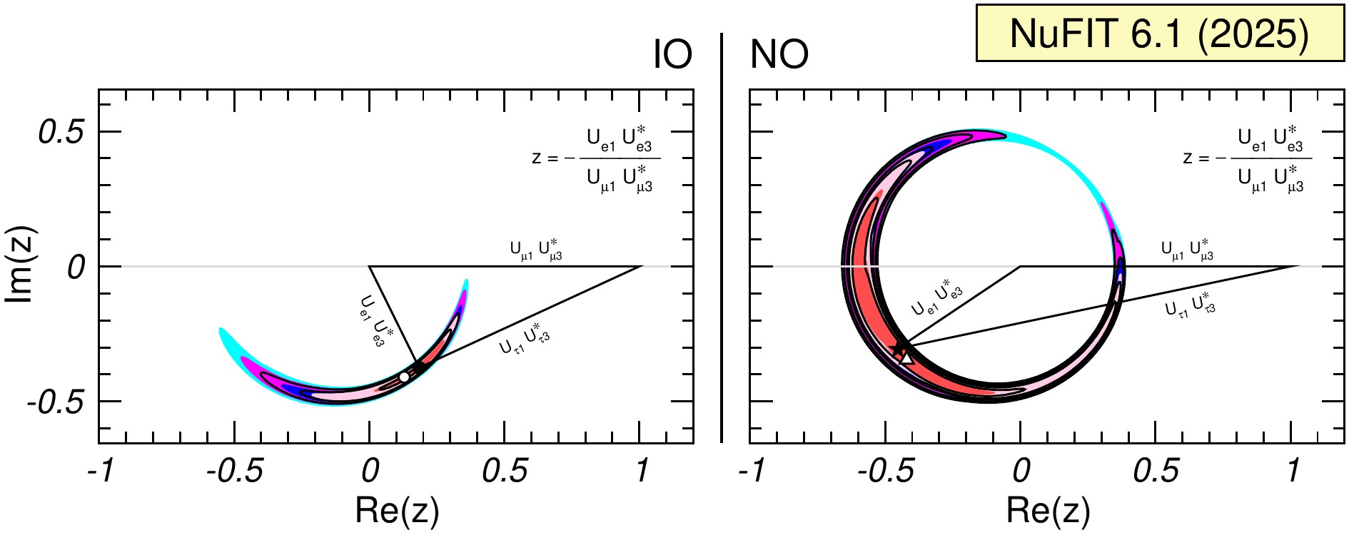
Allowed shapes of the leptonic unitarity triangle in NuFIT 6.1

\[ U_{e1}U_{\mu1}^*+U_{e2}U_{\mu2}^*+U_{e3}U_{\mu3}^*=0. \]

Three complex terms close a triangle. In the NuFIT figure, the closure is imposed in advance, and the triangle shapes allowed in the unitary model are shown. For a direct test, the closure is left free.
What remains to be checked

What to look for in the formulas

  • In \(P_{\alpha\to\alpha}\), the moduli of the elements of one row set the depth of disappearance, while \(\Delta m_{ij}^2\) sets the position of the maxima.
  • In \(P_{\alpha\to\beta}\) at \(\alpha\ne\beta\), products of different rows appear; the comparison of neutrinos and antineutrinos is sensitive to their imaginary parts.
  • Unitarity links the channels. Testing it independently requires relaxing these links in the data analysis.

The next lecture will begin with a question: how does matter change the phases of the neutrinos passing through it?

Exercises for Lecture 10 · Flavor triangle (in Russian) · Assemble the matrix (in Russian).

Exercises for this lecture

  • 10.1. Build the matrix from three hints
  • 10.2. How to read the PMNS matrix
  • 10.3. General three-flavor probability
  • 10.4. CP violation and the Jarlskog invariant
  • 10.5. Numerical lab of three flavors
  • 10.6. What the moduli of the matrix know about the phase \(\delta_{\mathrm{CP}}\)
  • 10.7. Two scales: when three flavors reduce to two
  • 10.8. Mass ordering in the reactor antineutrino spectrum
  • 10.9. The unitarity triangle and the number of phases