Neutrino Oscillations in Vacuum. Two Flavors
Introduction to Neutrino Physics
JINR
In Plain Words
Problem Statement
- In the Standard Model: \[ \begin{aligned} \text{possible}\qquad W^+\longrightarrow\ell_\alpha^++\nu_\alpha, \qquad&\overset{L=0}{\longrightarrow}\qquad \nu_\alpha+W^-\longrightarrow\ell_\alpha^-. \\ \text{impossible}\qquad W^+\longrightarrow\ell_\alpha^++\nu_\alpha, \qquad&\overset{L=0}{\longrightarrow}\qquad \nu_\alpha+W^-\longrightarrow\ell_\beta^-, \qquad \alpha\neq\beta. \end{aligned} \]
- If \(L\ne 0\), \(m_i \ne m_j\) and \(\theta\ne 0\), then the impossible becomes possible: \[ \text{possible}\qquad W^+\longrightarrow\ell_\alpha^++\nu_\alpha, \qquad\overset{L\ne 0}{\longrightarrow}\qquad \nu_\alpha+W^-\longrightarrow\ell_\beta^-, \qquad \alpha\neq\beta. \]
- The probability of such processes is a (quasi)periodic function of the ratio \(L/E\): \[ \boxed{P_{\alpha\to\beta}(L/E)}. \]
- This phenomenon is called neutrino oscillations.
Quantum Chameleon
Periodicity Is in the Probabilities
The two components acquire different phases. Their sum at detection determines the probabilities of the flavor outcomes.
Two Bases
Flavor at Birth, Mass in Flight
Weak interaction
\[ W^+\longrightarrow\ell_\alpha^++\nu_\alpha, \qquad \nu_\beta+N\longrightarrow\ell_\beta^-+X. \]
The charged lepton defines the flavor basis for production and detection.
Free propagation
\[ H_0|\nu_i\rangle=E_i|\nu_i\rangle, \qquad i=1,2. \]
The mass states are the eigenstates of the free Hamiltonian.
Both bases describe the same state space. Between them stands the mixing angle \(\theta\).
One Angle Connects the Two Bases
\[ \boxed{ \begin{pmatrix} |\nu_\alpha\rangle\\[2pt] |\nu_\beta\rangle \end{pmatrix} = \begin{pmatrix} \cos\theta&\sin\theta\\ -\sin\theta&\cos\theta \end{pmatrix} \begin{pmatrix} |\nu_1\rangle\\[2pt] |\nu_2\rangle \end{pmatrix}} \]
- At \(\theta=0\) each flavor coincides with one mass state.
- At \(\theta=\pi/4\) both mass states enter \(|\nu_\alpha\rangle\) with amplitudes of equal modulus.
To compute the transition we will need two rows of this rotation:
\[ |\nu_\alpha\rangle=c_\theta|\nu_1\rangle+s_\theta|\nu_2\rangle, \qquad |\nu_\beta\rangle=-s_\theta|\nu_1\rangle+c_\theta|\nu_2\rangle, \]
where \(c_\theta=\cos\theta\) and \(s_\theta=\sin\theta\).
Phases of the Two Eigenstates
\(\hbar=c=1\). The free Hamiltonian does not depend on time.
Let \(\varphi_i\) be the phase accumulated by a mass component between the source and the detector. Then
\[ |\nu_\alpha;t,L\rangle =c_\theta e^{-i\varphi_1}|\nu_1\rangle +s_\theta e^{-i\varphi_2}|\nu_2\rangle. \]
If the initial state contains a single eigenstate, the phase factor disappears when the probability is computed. Here two waves are present; after factoring out the common factor, the difference remains:
\[ \boxed{\Delta\varphi=\varphi_2-\varphi_1}. \]
As it accumulates, the result of adding the amplitudes at the detector changes.
Projection onto the Other Flavor
The detector looks for the state \(|\nu_\beta\rangle\). We project the evolved state onto it:
\[ \begin{aligned} \mathcal A_{\alpha\to\beta} &=\langle\nu_\beta|\nu_\alpha;t,L\rangle\\ &=(-s_\theta\langle\nu_1|+c_\theta\langle\nu_2|) \left(c_\theta e^{-i\varphi_1}|\nu_1\rangle +s_\theta e^{-i\varphi_2}|\nu_2\rangle\right). \end{aligned} \]
The mass states are orthonormal: \(\langle\nu_i|\nu_j\rangle=\delta_{ij}\). Two contributions remain:
\[ \boxed{ \mathcal A_{\alpha\to\beta} =s_\theta c_\theta \left(e^{-i\varphi_2}-e^{-i\varphi_1}\right) }. \]
At \(L=0\) the phases are equal, and the two contributions cancel. Further on they diverge.
We use
\[ \left|e^{-i\varphi_2}-e^{-i\varphi_1}\right|^2 =4\sin^2\frac{\Delta\varphi}{2}, \qquad 4s_\theta^2c_\theta^2=\sin^22\theta. \]
By the Born rule
\[ \boxed{ P_{\alpha\to\beta}(t,L) =\sin^22\theta\, \sin^2\frac{\Delta\varphi(t,L)}{2} }. \]
Two Possible Outcomes
In the two-flavor model the probabilities exhaust all detection possibilities:
\[ \boxed{P_{\alpha\to\alpha}=1-P_{\alpha\to\beta}}. \]
- For a nonzero mass splitting, the angle \(\theta\) sets the height of the maxima: \(P_{\alpha\to\beta}^{\max}=\sin^22\theta\).
- The phase difference sets the positions of the maxima and minima.
- At the point \(L=0\) we obtain \(P_{\alpha\to\beta}=0\) and \(P_{\alpha\to\alpha}=1\).
From Time to Distance
Phase Along the Path
For a plane wave moving along the \(L\) axis,
\[ e^{-i\varphi_i(t,L)}=e^{-i(E_it-p_iL)}, \qquad \varphi_i(t,L)=E_it-p_iL. \]
Here \(p_i\) is the momentum along the direction from the source to the detector.
Hence,
\[ \boxed{\Delta\varphi(t,L)=\Delta E\,t-\Delta p\,L}, \qquad \Delta E=E_2-E_1, \quad \Delta p=p_2-p_1. \]
The detector is located at a distance \(L\). For an ultrarelativistic neutrino, the flight time \(t\simeq L\) in units of \(c=1\). Both components must remain coherent until detection.
From Mass to Phase
We use the dispersion relation of each mass wave:
\[ E_i^2-p_i^2=m_i^2 \quad\Longrightarrow\quad E_i-p_i=\frac{m_i^2}{E_i+p_i}. \]
For \(t\simeq L\) and \(E_i\simeq p_i\simeq E\), to leading order:
\[ \varphi_i(t,L) \simeq(E_i-p_i)L \simeq\frac{m_i^2L}{2E}. \]
Therefore
\[ \boxed{ \Delta\varphi\simeq\frac{\Delta m^2L}{2E}}, \qquad \Delta m^2=m_2^2-m_1^2. \]
Probability at Distance \(L\)
The argument of the sine contains half of the relative phase:
\[ \boxed{ P_{\alpha\to\beta}(L,E) =\sin^22\theta\, \sin^2\left(\frac{\Delta m^2L}{4E}\right) }. \]
The period in distance at fixed energy is
\[ \boxed{L_{\rm osc}=\frac{4\pi E}{|\Delta m^2|}}. \]
The first transition maximum occurs at \(L=L_{\rm osc}/2\).
What the Plot Shows
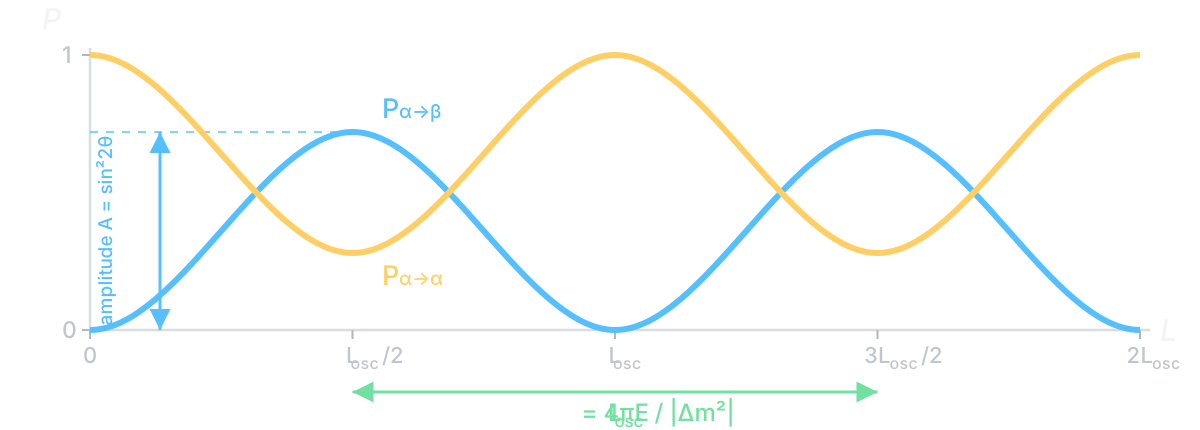
- The height of the maximum gives \(\sin^22\theta\).
- The distance between neighboring maxima, for a known \(E\), gives \(|\Delta m^2|\).
Checking the Formula
Build the Oscillation Yourself
A = sin²2θ = 0.750
- Set \(\theta=0\): how does the curve change?
- Set \(\theta=45^\circ\): find the first maximum.
- Move \(L/L_{\rm osc}\) from \(0\) to \(1\): where does the transition probability return to zero?
Mechanical Model
Two Pendulums of Different Masses
P₁ + P₂ = 1 exactly, no averaging
Two Frequencies in One Mechanical System
We excite one pendulum
The initial displacement decomposes into two normal modes. Each mode oscillates with its own frequency \(\omega_+\) or \(\omega_-\).
We observe both pendulums
The relative phase \((\omega_--\omega_+)t\) changes. The envelope of the motion periodically shifts from one pendulum to the other.
\[ \boxed{ P_{1\to2}(t)=\sin^22\theta\, \sin^2\!\left(\frac{(\omega_--\omega_+)t}{2}\right) }. \]
Here \(P_i\) are the normalized squared moduli of the complex amplitudes of the local pendulums. For weak coupling they are approximately equal to the fractions of the averaged energy. The exact derivation is in Exercise 9.6.
Two Flavors
The Formula and Its Physical Meaning
\[ \boxed{ P_{\alpha\to\beta}(L,E) =\sin^22\theta\, \sin^2\!\left(\frac{\Delta m^2L}{4E}\right) }. \]
- The weak interaction prepares and measures the flavor.
- The mass components acquire different phases during propagation.
- The interference of these components determines the fraction of events with flavor \(\beta\).
In the next lecture a third state will be added to the two mass states.
Exercises for Lecture 09 · Two-flavor applet (in Russian) · Coupled pendulums applet (in Russian).
Exercises for this lecture
- 9.1. Global and relative phases
- 9.2. Energy of a flavor state
- 9.3. Complete derivation of the two-flavor probability
- 9.4. From the plane-wave phase to the dependence on L/E
- 9.5. A mock-up of an oscillation experiment
- 9.6. Coupled pendulums of different masses
- 9.7. Oscillation scales: from a reactor to the Sun
- 9.8. Averaging of oscillations and the 1/2 bound
- 9.9. When the mass components stop interfering