viewof cresModulationIndex = Inputs.range([0, 4], {
  value: 1.2,
  step: 0.1,
  label: html`
    <span class="spectrum-slider-label">
      ${tex`h=\Delta f/f_z`}
    </span>
  `
})

cresAxialFrequency = 25
cresObservationTime = 80
cresSpectrumOrders = Array.from({length: 29}, (_, i) => i - 14)

cresFactorial = n => {
  let value = 1
  for (let k = 2; k <= n; ++k) value *= k
  return value
}

cresBesselPositive = (n, x) => {
  let value = 0
  for (let k = 0; k < 24; ++k) {
    value += ((k % 2 === 0) ? 1 : -1)
      * Math.pow(x / 2, 2 * k + n)
      / (cresFactorial(k) * cresFactorial(k + n))
  }
  return value
}

cresBessel = (n, x) => {
  const order = Math.abs(n)
  const value = cresBesselPositive(order, x)
  return n < 0 && order % 2 === 1 ? -value : value
}

cresLineWeights = cresSpectrumOrders.map(order => ({
  order,
  frequency: order * cresAxialFrequency,
  amplitude: cresBessel(order, cresModulationIndex),
  power: Math.pow(cresBessel(order, cresModulationIndex), 2)
}))

cresSinc = value => Math.abs(value) < 1e-12
  ? 1
  : Math.sin(value) / value

cresFrequencyGrid = Array.from({length: 1201}, (_, i) => -150 + i / 4)
cresSpectrum = cresFrequencyGrid.map(frequency => ({
  frequency,
  power: (() => {
    let real = 0
    let imaginary = 0
    for (const line of cresLineWeights) {
      const argument = Math.PI
        * (frequency - line.frequency)
        * 1000
        * cresObservationTime
        * 1e-6
      const amplitude = line.amplitude * cresSinc(argument)
      real += amplitude * Math.cos(argument)
      imaginary -= amplitude * Math.sin(argument)
    }
    return real * real + imaginary * imaginary
  })()
}))

cresSpectrumMaximum = Math.max(...cresSpectrum.map(point => point.power))
cresNormalizedSpectrum = cresSpectrum.map(point => ({
  frequency: point.frequency,
  power: point.power / cresSpectrumMaximum
}))

cresNormalizedLines = cresLineWeights.map(line => ({
  frequency: line.frequency,
  power: line.power / Math.max(...cresLineWeights.map(item => item.power))
}))

cresSpectrumPlot = Plot.plot({
  width: 1040,
  height: 260,
  marginTop: 6,
  marginRight: 25,
  marginBottom: 30,
  marginLeft: 72,
  style: {
    background: "#ffffff",
    color: "#111111",
    fontSize: "18px"
  },
  x: {
    axis: "bottom",
    label: null,
    domain: [-150, 150],
    ticks: 7,
    grid: true
  },
  y: {
    axis: "left",
    label: null,
    domain: [0, 1.05],
    ticks: 3,
    grid: true
  },
  marks: [
    Plot.line(cresNormalizedSpectrum, {
      x: "frequency",
      y: "power",
      stroke: "#4ea1ff",
      strokeWidth: 3
    }),
    Plot.ruleX(cresNormalizedLines.filter(line => Math.abs(line.frequency) <= 150), {
      x: "frequency",
      y1: 0,
      y2: "power",
      stroke: "#ffb347",
      strokeWidth: 3
    }),
    Plot.frame({stroke: "#111111"})
  ]
})

html`
<div class="spectrum-panel">
  <div class="spectrum-plot-row">
    <div class="spectrum-y-label">${tex`(dP/df)_{\rm norm}`}</div>
    <div class="spectrum-plot-host">${cresSpectrumPlot}</div>
  </div>
  <div class="spectrum-x-label">${tex`f-f_c\;(\text{kHz})`}</div>
  <div class="spectrum-summary">
    <span>${tex`f_z=${cresAxialFrequency}\ \text{kHz}`}</span>
    <span>${tex`T_{\rm obs}=${cresObservationTime}\ \mu\text{s}`}</span>
    <span>${tex`\Delta f_{\rm FWHM}\simeq0.886/T_{\rm obs}\simeq${(886 / cresObservationTime).toFixed(1)}\ \text{kHz}`}</span>
  </div>
</div>`Direct Determination of the Neutrino Mass.
Other Ways to Weigh the Neutrino
Introduction to Neutrino Physics
Energy can be converted into frequency or heat
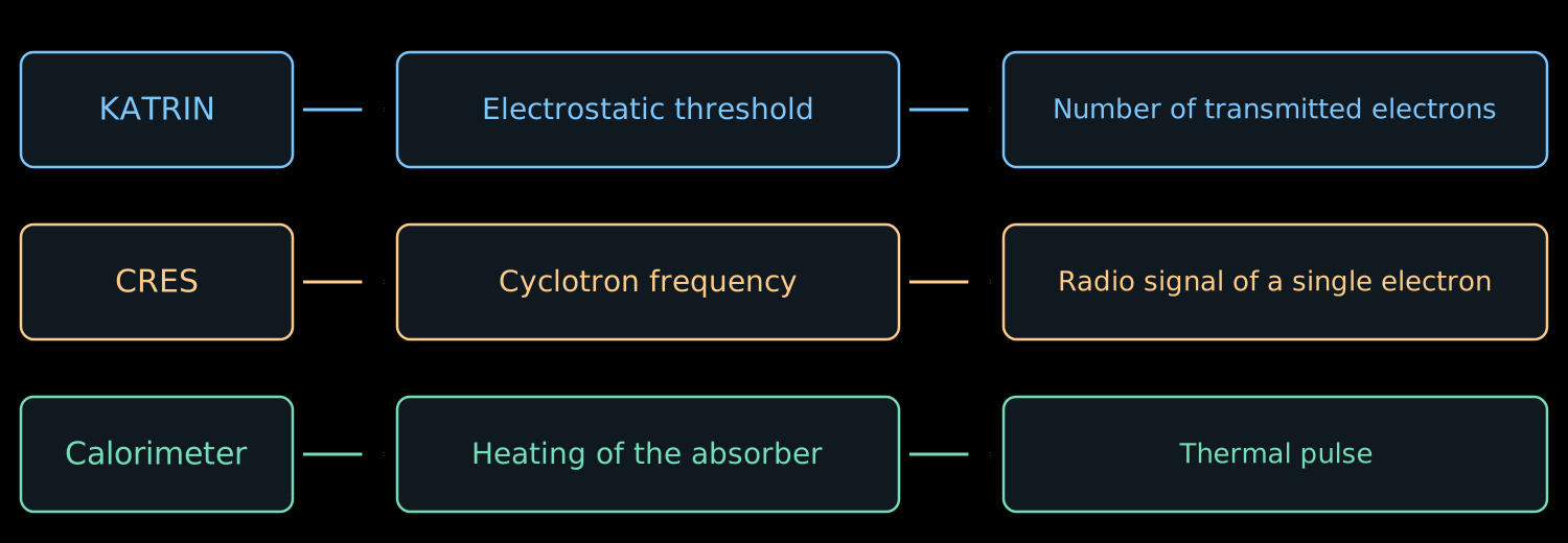
- In lecture 07 we measured several integrals of the \(\beta\) spectrum by varying the retarding voltage.
- Now we consider ways to measure the energy of each decay individually.
- There will be four ways:
- hear the electron;
- measure the heat;
- reconstruct the missing momentum;
- compare arrival times.
The cyclotron frequency depends on energy
- The energy does not appear in the nonrelativistic formula \(\omega_c=eB/m_e\).
- In lecture 05 we obtained the relativistic refinement:
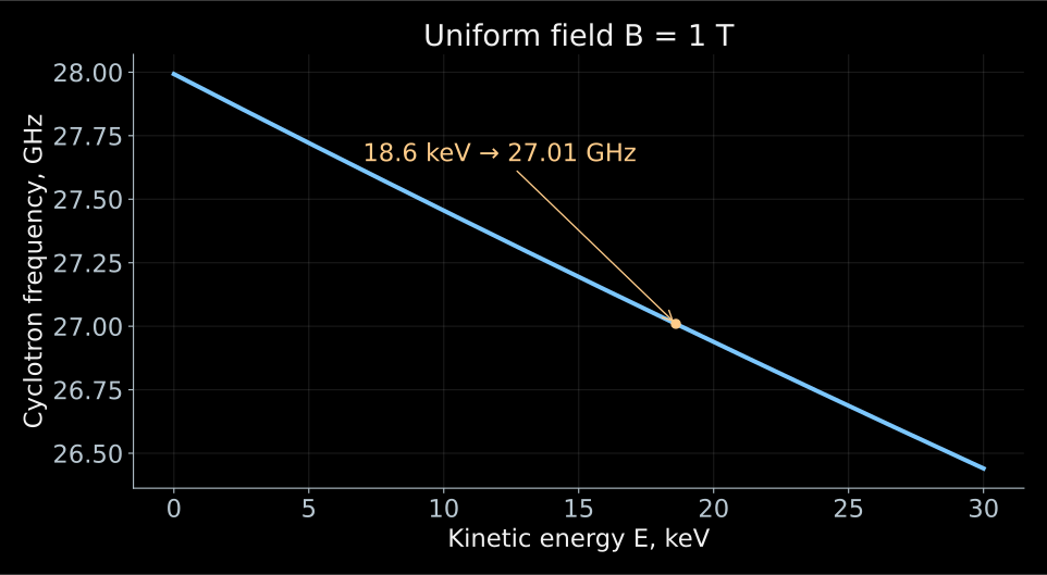
\[ f_c=\frac{\omega_c}{2\pi} =\frac{eB}{2\pi\gamma m_e} =\frac{f_0}{\gamma}, \qquad \gamma=1+\frac{E}{m_ec^2}. \]
- Here \(f_0=eB/(2\pi m_e)\). A more energetic electron rotates more slowly.
- If the field is known, the frequency gives the energy:
\[ \boxed{E=m_ec^2\left(\frac{f_0}{f_c}-1\right)}. \]
- The electron moves with acceleration transverse to the magnetic field and emits an electromagnetic wave.
- The periodic rotation creates a signal at the cyclotron frequency. It can be received for as long as the electron remains in the observed volume.
- For \(B=1\) T and \(E=18.6\) keV
\[ f_0\simeq27.99~\text{GHz}, \qquad f_c\simeq27.01~\text{GHz}. \]
- This approach is called cyclotron radiation emission spectroscopy, abbreviated CRES. It is being developed by the Project 8 experiment.
In the electrodynamic formulas of this lecture \(c\) is written explicitly, and \(E\) is the kinetic energy of the electron. Principle and implementation of CRES.
What arrives at the receiver input?
- In the free-space approximation the radiated power is
\[ P_{\mathrm{rad}} =\frac{e^4B^2}{6\pi\varepsilon_0m_e^2c} \,\gamma^2\beta^2\sin^2\alpha. \]
- \(\beta=v/c\), \(\alpha\) is the angle between the velocity and the field. The transverse acceleration radiates; for \(\alpha=0\) there is no cyclotron radiation.
- For \(E=18.6\) keV, \(B=1\) T, \(\alpha=90^\circ\):
\[ \boxed{P_{\mathrm{rad}}\simeq1.2\cdot10^{-15}~\text{W}}. \]
- Only part of the power reaches the receiver. A waveguide or a resonator changes both the collection of the signal and the conditions of the emission itself.
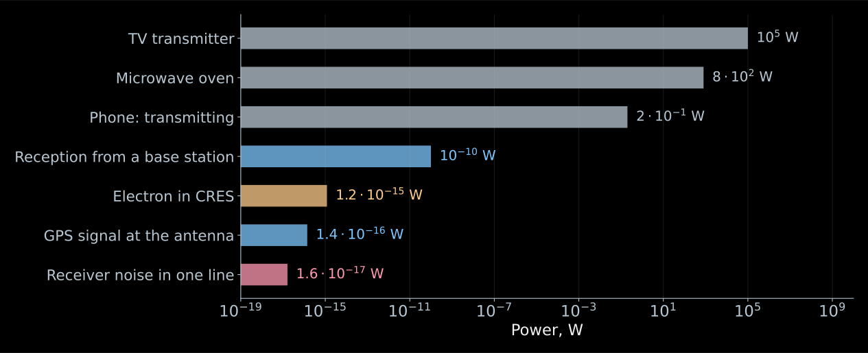
- A phone during transmission radiates \(0.2\) W, a cell tower hundreds of kilowatts.
- The antenna of the same phone receives about \(10^{-10}\) W from the base station.
- The GPS signal at this antenna is \(1.4\cdot10^{-16}\) W, and it is reliably received by every smartphone.
- Our femtowatt lies above the GPS signal.
Comparing our femtowatt with transmitters is meaningless. What does it actually compete with?
- There is only one competitor: the thermal noise of the receiver itself. It gives a power \(kT_{\mathrm{n}}\) per hertz of bandwidth.
- The bandwidth is set by the recording duration: the longer we listen to the electron, the narrower the line in the spectrum,
\[ \Delta f\simeq\frac{0.886}{T_{\mathrm{obs}}}. \]
- For \(T_{\mathrm{n}}=132\) K and a recording of length \(100\) μs, the noise in one such line is
\[ \boxed{ P_{\mathrm{n}}=kT_{\mathrm{n}}\,\Delta f \simeq1.6\cdot10^{-17}~\text{W} }. \]
- A femtowatt against this is a margin of almost a factor of one hundred. Part of the power is lost on the way to the amplifier, and the working signal-to-noise ratio comes out at a few units.
Listen for a long time and in a narrow band.
How the receiving chain is built
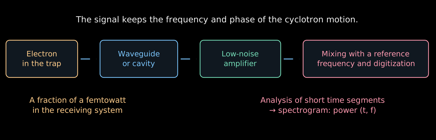
- The electron gives up its power to an electromagnetic mode, and the mode delivers it to the amplifier.
- The amplifier raises the level, the mixer lowers the frequency, and the ADC records the voltage as a function of time.
- Each step preserves the frequency, the very quantity for the sake of which everything is done.
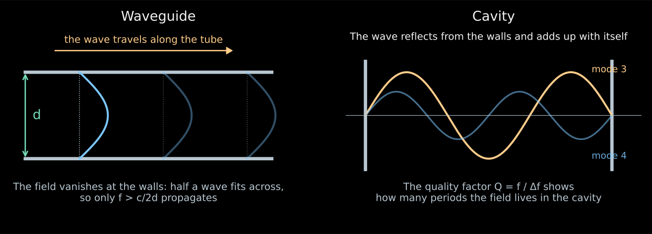
- A resonator is a closed cavity. The wave is reflected from the walls and adds up with itself at selected frequencies.
- The quality factor \(Q=f/\Delta f\) counts how many periods the field lives in the cavity. For \(Q=10^4\) at \(26\) GHz the resonator bandwidth is \(2.6\) MHz.
- A waveguide is a metal tube. The field vanishes at the walls, so at least a half-wave must fit across the tube:
\[ f>f_{\mathrm{cr}}\simeq\frac{c}{2d}. \]
- For \(d=10\) mm this is \(15\) GHz; an exact calculation for a circular tube gives \(17.6\) GHz. A signal at \(26\) GHz passes, while everything below the cutoff is attenuated.
- The femtowatts must be raised to a level that will survive cables and digitization. The gain in Project 8 is from \(70\) to \(82\) dB, that is, a factor of \(10^7\)–\(10^8\) in power.
- This has to be paid for: the amplifier adds its own noise. It is expressed by the temperature \(T_{\mathrm{n}}\), and the noise power is \(kT_{\mathrm{n}}\) per hertz of bandwidth.
- For a chain of stages with gains \(G_i\)
\[ \boxed{ T_{\mathrm{sys}}=T_1+\frac{T_2}{G_1}+\frac{T_3}{G_1G_2}+\ldots } \]
- The noise of the first stage enters in full, while the others are divided by the gain of the preceding ones. This is why the first amplifier is cooled and everything else is tolerated.
- For Project 8, \(T_{\mathrm{sys}}=132\) K.
- There is nothing to record \(26\) GHz directly. The mixer multiplies the signal by a reference oscillation of frequency \(f_{\mathrm{ref}}\):
\[ \cos(2\pi f_ct)\cos(2\pi f_{\mathrm{ref}}t) =\frac12\cos[2\pi(f_c-f_{\mathrm{ref}})t] +\frac12\cos[2\pi(f_c+f_{\mathrm{ref}})t]. \]
- A filter keeps the difference. Mixing \(26\) GHz with \(24.5\) GHz, we get \(1.5\) GHz; all frequency changes are preserved in this shift without distortion.
- The ADC records the voltage at a sampling rate above twice the bandwidth, otherwise different frequencies become indistinguishable.
- Fourier analysis of short pieces of the recording gives a spectrogram: the power as a function of time and frequency.
A single electron leaves a frequency track
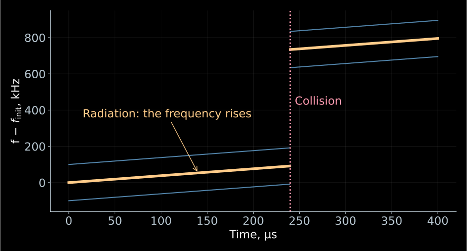
- A schematic track at constant average field.
- The loss in a single collision is chosen to be \(12.6\) eV;
- the side lines are shown schematically.
- Time is on the horizontal axis, frequency on the vertical.
- The start of the first detected line gives an estimate of the initial energy of the electron.
- The smooth rise is due to the loss of energy to radiation:
\[ \dot E=-P_{\mathrm{rad}}, \qquad \dot f_c=\frac{f_cP_{\mathrm{rad}}}{m_ec^2+E}>0. \]
- A collision with a molecule can sharply reduce the energy: the frequency will jump up.
- Neighboring lines may belong to the same electron.
- In lectures 05–06 the Lorentz force did no work: \(q\mathbf v\cdot(\mathbf v\times\mathbf B)=0\).
- But there we neglected radiation. Now it is the observable signal and carries away the electron’s energy.
- The magnetic field does not supply this energy. The electron spends its own kinetic energy; in the exact equation of motion a radiation reaction force appears.
- At a power of \(1.2\) fW, over \(100\) μs approximately the following is lost:
\[ P_{\mathrm{rad}}T_{\mathrm{obs}} \simeq1.2\cdot10^{-19}~\text{J} \simeq0.75~\text{eV}. \]
- Therefore the initial energy is reconstructed from the start of the track, taking into account its subsequent evolution.
- The electron is held in the trap; the radiation produces a rising track. A collision changes its frequency.
A schematic animation; its notation \(K\) corresponds to the kinetic energy \(E\) in the lecture.
The magnetic mirror prolongs the observation
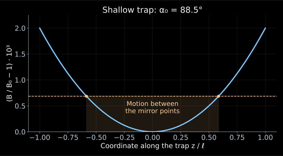
- Without a trap the electron would quickly leave the sensitive region.
- Two magnetic mirrors reflect it back, using the effect of lecture 06.
- Between reflections the energy changes little over one longitudinal period, and the adiabatic invariant can be applied.
- If the field at the edges is only slightly larger than \(B_0\), electrons with angles close to \(90^\circ\) are trapped:
\[ \boxed{\sin^2\alpha_0>\frac{B_0}{B_{\max}}}. \]
- Let \(B_{\max}=B_0(1+\eta)\), where \(\eta\ll1\) is the relative depth of the trap.
- The trapping condition takes the form
\[ |\cos\alpha_0|< \sqrt{1-\frac{1}{1+\eta}} \simeq\sqrt{\eta}. \]
- For an isotropic source \(\cos\alpha_0\) is uniform on \([-1,1]\). Therefore the geometric fraction of trapped electrons is approximately \(\sqrt{\eta}\).
- A deep trap accepts more angles, but the electron explores a larger range of fields.
- The frequency depends on both the energy and the field: the gain in statistics complicates the reconstruction of the energy.
- The trap field is constant in time. The electron moves, and along with it the field changes at the point where it is currently located.
- In the parabolic approximation
\[ B(z)=B_0\left(1+\frac{z^2}{\ell^2}\right), \qquad z(t)=z_{\max}\cos(2\pi f_zt). \]
- Substitution gives
\[ B(t)=B_0\left[ 1+\frac{z_{\max}^2}{2\ell^2} +\frac{z_{\max}^2}{2\ell^2}\cos(4\pi f_zt) \right]. \]
- Over one longitudinal period the electron twice enters the region of strong field, so the rotation frequency oscillates at \(2f_z\).
- The average frequency also shifts. Substituting a single \(B_0\) into the formula for \(E\) without a correction for the trajectory will give an error.
Why does a single electron produce several lines?
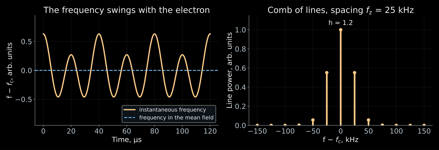
The total phase of the received signal is the sum of the rotation phase and the wave delay, \(\Phi_{\mathrm{rec}}(t)=\int_0^t2\pi f_c\,dt'+\Phi_{\mathrm{prop}}[z(t)]\): the first term oscillates at \(2f_z\), the second at \(f_z\). CRES power spectrum and axial motion.
- The electron oscillates between the mirrors with frequency \(f_z\) and twice per period enters the strong field. The cyclotron frequency oscillates along with it.
- At the same time, the distance to the receiver changes: the wave arrives sometimes slightly earlier, sometimes slightly later.
- The receiver hears a sinusoid whose period slightly “breathes” with period \(1/f_z\).
- This breathing of the phase splits a single line into a comb:
\[ \boxed{f_n=f_c+nf_z}. \]
- All these lines belong to a single electron.
- First, let us keep only one modulation frequency:
\[ V(t)=V_0\cos\Phi(t), \qquad \Phi(t)=2\pi f_ct+h\sin(2\pi f_zt). \]
- The instantaneous frequency is determined by the derivative of the phase:
\[ f_{\mathrm{inst}}=\frac{1}{2\pi}\frac{d\Phi}{dt} =f_c+h f_z\cos(2\pi f_zt). \]
- Hence \(h=\Delta f/f_z\) is the dimensionless modulation index, and \(\Delta f\) is the amplitude of the frequency variation.
- For small \(h\) the signal is nearly harmonic. For large \(h\) the sidebands carry a noticeable fraction of the power.
- The Jacobi–Anger identity gives
\[ e^{ih\sin\theta}=\sum_{n=-\infty}^{\infty}J_n(h)e^{in\theta}. \]
- Consequently,
\[ e^{i\Phi(t)} =\sum_{n=-\infty}^{\infty}J_n(h)e^{2\pi i(f_c+nf_z)t}. \]
- \(J_n\) is the Bessel function. The sideband has frequency \(f_n=f_c+nf_z\) and relative power \(J_n^2(h)\).
- For a long observation
\[ \sum_nJ_n^2(h)=1: \]
the power is redistributed among the lines and does not vanish.
- The comb takes power away from the central line. The detection threshold has to be computed for the line that we actually see.
- The spacing between the lines equals \(f_z\). It depends on the pitch angle and on how deeply the electron penetrates into the trap, and thus tells us about the trajectory.
- The trajectory determines the average field along the path, and without it the frequency cannot be converted into energy.
- At \(h\approx2.4\) the function \(J_0\) vanishes: the central line is extinguished, although the electron has not gone anywhere.
From individual tracks to the Project 8 spectrum
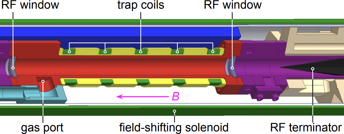
- The electron is born in the decay right inside the waveguide and remains there, confined by the trap coils.
- The radio wave travels along the pipe to the amplifiers, and at the far end it is absorbed by a terminator so that no echo returns.
- The gas is supplied through a separate inlet, and the field-shifting solenoid changes the operating field without retuning the magnet itself.
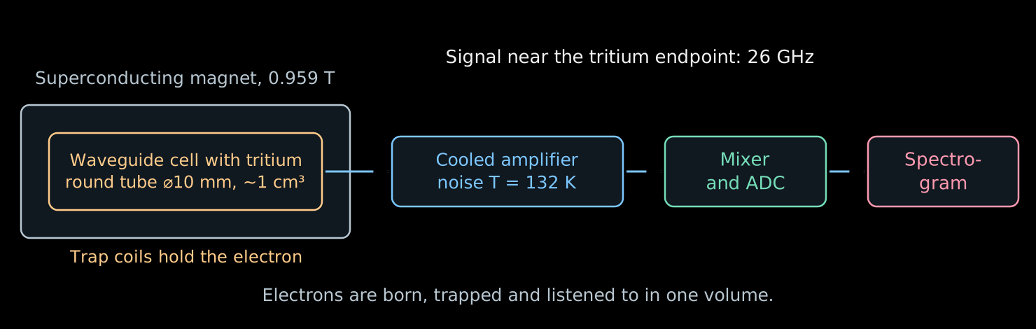
| Parameter | Value |
|---|---|
| Field | \(0.959\) T |
| Frequency at the endpoint of the spectrum | \(\simeq26\) GHz |
| Cell | circular waveguide \(\varnothing\,10\) mm |
| Volume | of order cm³ |
| System noise | \(132\) K |
| Gain | \(70\)–\(82\) dB |
| Resolution on the Kr line | \(1.66\) eV |
Phase II parameters. Overview of the method and the apparatus.
- For each detected electron the start of the track is reconstructed.
- The initial frequencies are converted into energies and used to fill the spectrum. It is then compared with a model of β decay and of the response.
- Not every electron produces a visible track: the detection probability depends on the power, duration, angle, and the receiver bandwidth.
- If the first segment is too weak or too short, the electron may be noticed only after it has lost energy. This distorts the reconstructed spectrum.
- Calibrations and an efficiency model are needed here just as in KATRIN.
Project 8: the first measurement and next steps
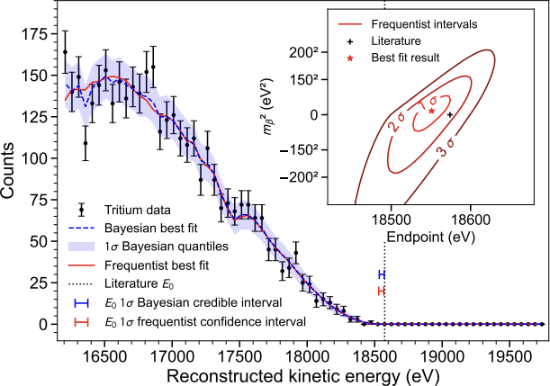
Figure 5 and the result: Project 8, Phys. Rev. Lett. 131, 102502 (2023).
- In 2023 Project 8 published the first tritium spectrum measured via cyclotron radiation.
- The following limits were obtained:
\[ m_\beta<155~\text{eV}\quad(90\%\ \text{Bayesian interval}), \]
\[ m_\beta<152~\text{eV}\quad(90\%\ \text{frequentist interval}). \]
- A resolution of \(1.66\pm0.19\) eV FWHM was demonstrated on the line \(^{83\mathrm m}\mathrm{Kr}\) at about \(17.8\) keV in a specially chosen shallow trap.
- Good resolution for a single electron does not yet give a strong limit on the mass: the number of tritium events and the full response matter.
- The source volume is one cubic centimeter. The KATRIN source is ten meters long, hence the difference in the limits: \(155\) eV versus \(0.45\) eV.
- Phase II solved its own problem: to demonstrate the resolution. With a single electron, \(1.66\) eV was obtained in a volume the size of a thimble.
- Next, volume is needed. The weak signal is collected either with an antenna array, adding the signals with delays according to the electron position, or with a resonator with a chosen mode.
- Phase III is a resonator on the m³ scale. Phase IV is atomic tritium with a goal of \(40\) meV.
- CRES will begin to measure the physics of the neutrino mass in the subsequent phases.
- In molecular tritium part of the energy remains in the rotation and vibration of the daughter molecule. Frequency readout by itself does not eliminate this.
- Atomic tritium removes the molecular degrees of freedom, but retains atomic excitations and recoil.
- The atoms must be cooled, trapped, and protected from recombination into molecules on the walls.
- The goal discussed for Project 8 is a sensitivity of order \(40\) meV. This requires a large atomic source and a new readout.
Calorimeter: the big picture
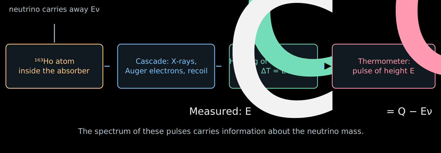
- The \(^{163}\mathrm{Ho}\) atom sits inside the absorber and captures its own electron. The neutrino escapes, and the rest stays right here.
- The X-ray quanta and Auger electrons of the cascade are stopped in the material, and within microseconds all of this turns into heat.
- The absorber heats up, the thermometer converts the temperature rise into a pulse, and the pulse height gives
\[ \boxed{E_c=Q-E_\nu}. \]
- \(Q\) is the total energy release of the decay, \(E_c\) is the measured calorimetric energy.
- Next we will examine each link of this chain separately.
Electron capture in holmium-163
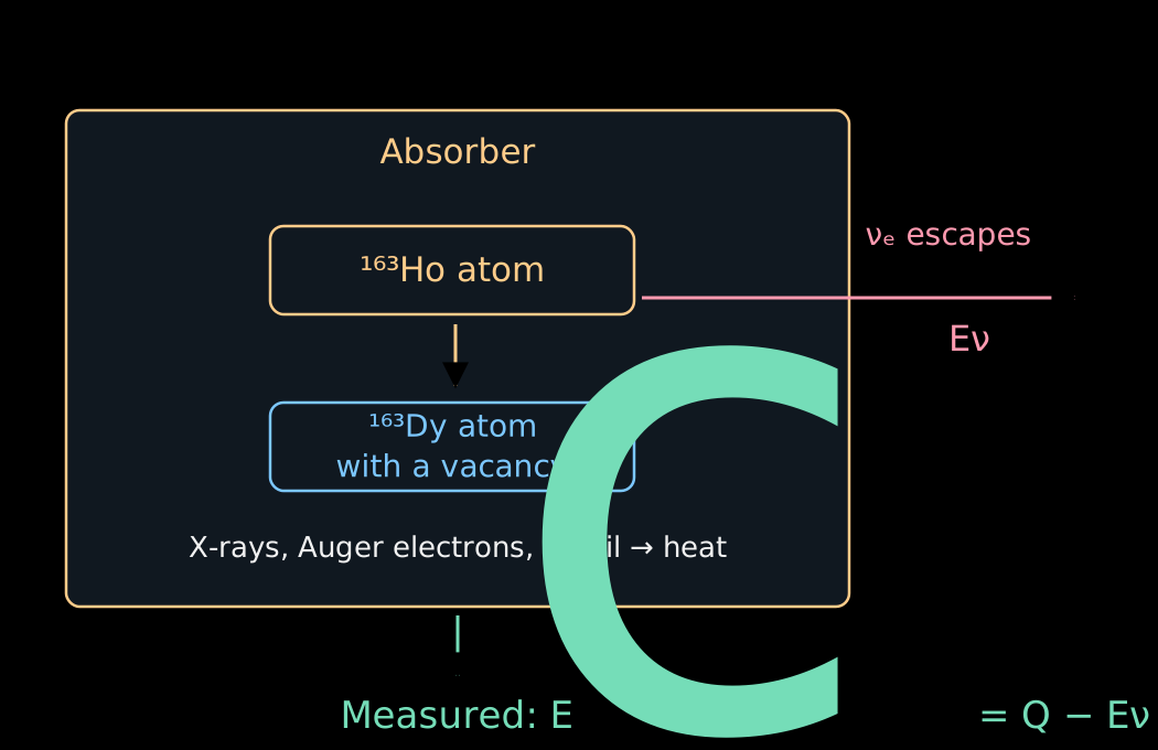
- A proton of the nucleus captures one of the bound electrons of its atom:
\[ p+e^-_{\mathrm{b}}\to n+\nu_e. \]
- The nuclear charge decreases by one. For the complete neutral atom
\[ {}^{163}\mathrm{Ho}_{\mathrm{at}} \to{}^{163}\mathrm{Dy}_{\mathrm{at}}^*+\nu_e. \]
- Here the asterisk denotes an excitation of the electron shell: after the capture a vacancy remains and the field of the nucleus has been rearranged.
- The mass difference of the neutral atoms sets \(Q\simeq2.86\) keV. The bound electron is already included in the mass of the initial atom.
- An electron from an outer shell can fill the vacancy.
- The released energy is emitted as an X-ray quantum or transferred to another electron, which leaves the atom. The latter process produces an Auger electron.
- A cascade of shell rearrangements arises. Inside the absorber all of these particles transfer their energy to the material.
- The calorimeter sums the cascade. For the same final atomic state, it does not matter how the energy was shared between photons and electrons.
The calorimeter measures the total remaining energy, even if it was spread among several particles.
- Photons and electrons must be absorbed inside the sensitive volume. The escape of a photon would reduce the measured energy and create a tail in the response.
- The energy must have time to pass into the measurable thermal degrees of freedom. Long-lived excitations can change the pulse shape.
- The positions of the implanted atoms, the absorber thickness and the calibration are checked experimentally.
- When these conditions are met, the losses due to electron escape from a separate source, familiar from lecture 07, disappear.
Why does the calorimetric spectrum contain peaks?
- The electron can be captured from different shells. After the capture, different excitation energies of the dysprosium atom remain.
- For a perfectly defined final state, the two-body kinematics would give one neutrino energy and one \(E_c\).
- But excited atomic states have a finite lifetime and a natural width.
- Several channels give several lines with tails. Additional excitations and ionization of other electrons complicate the spectrum.
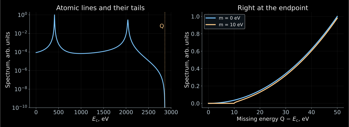
- The atomic peaks account for most of the statistics. The sensitivity to a small mass lies near the endpoint \(E_c\simeq Q\).
A teaching two-line spectrum. The mass \(10\) eV is chosen for illustration; these are not ECHo or HOLMES data.
- In the approximation of unresolved light masses we introduce \(x=Q-E_c\). For \(x\ge m_\beta\):
\[ \boxed{ \frac{d\Gamma}{dE_c} =C\,x\sqrt{x^2-m_\beta^2}\,\Theta(x-m_\beta)\,\mathcal A(E_c) }. \]
- \(C\) is a normalization, \(\mathcal A(E_c)\) is the atomic spectral function.
- The simplest model of independent lines:
\[ \mathcal A(E_c)\simeq \sum_j a_j\, \frac{\Gamma_j/(2\pi)} {(E_c-E_j)^2+\Gamma_j^2/4}. \]
- \(E_j\), \(\Gamma_j\), \(a_j\) are the energy, width and weight of a channel. The mass correction multiplies the entire atomic function.
- The single-vacancy model gives a useful picture, but is insufficient for a precise analysis of the end of the spectrum.
- After the change of the nuclear charge, the other electrons can additionally be excited or go into the continuum.
- Therefore \(\mathcal A(E_c)\) requires a many-electron calculation and a check against the measured lines.
- In the effective one-mass model the edge is \(E_c^{\max}=Q-m_\beta\). The exact three-mass description contains thresholds \(Q-m_i\) with weights \(|V_{ei}|^2\).
- A small \(Q\) is useful.
- The atomic peaks are needed to calibrate the detector and to test the spectrum model. To measure a small neutrino mass, sufficient statistics right at the endpoint of the spectrum are necessary.
How to measure the heating from a single decay?
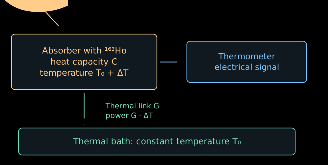
- The absorber is cooled to a temperature of the order of tens of millikelvin. Its heat capacity \(C\) becomes small.
- A rapid release of energy raises the temperature:
\[ \boxed{\Delta T\simeq\frac{E_c}{C}}. \]
- For example, for \(C=10^{-12}\) J/K the energy \(2.86\) keV gives
\[ \Delta T\simeq0.46~\text{mK}. \]
- The thermometer converts this temperature rise into an electrical signal.
- After the decay, the energy gradually flows into the thermal bath through the thermal link \(G\).
- In the linear model, once the energy release is over,
\[ C\frac{d\Delta T}{dt}=-G\Delta T. \]
- Hence
\[ \boxed{ \Delta T(t)=\frac{E_c}{C}e^{-t/\tau_{\mathrm{th}}}, \qquad \tau_{\mathrm{th}}=\frac{C}{G} }. \]
- A small \(C\) increases the amplitude, while a large \(G\) speeds up the return.
- The sensitivity is limited by the thermometer noise and thermal fluctuations. The speed and the energy resolution have to be chosen together.
Two ways to turn temperature into a signal
- ECHo uses metallic magnetic calorimeters. The sensor contains paramagnetic erbium ions in a metallic matrix.
- In a weak field the magnetic moments are partially ordered. Heating enhances the thermal disordering and decreases the magnetization.
- The simplest picture is the Curie law \(M\propto B/T\). A real sensor is calibrated at its operating temperature and field.
- The change of magnetic flux is read out by a SQUID — a superconducting quantum interference device, a sensitive magnetometer.
\[ E_c\ \longrightarrow\ \Delta T \ \longrightarrow\ \Delta M \ \longrightarrow\ \Delta\Phi. \]
- HOLMES uses sensors at the edge of the superconducting transition: TES is the accepted abbreviation for this type of thermometer.
- The sensor is held within a narrow temperature interval where the resistance changes sharply from almost zero to its normal value.
- A small heating noticeably raises the resistance. At a fixed voltage the current decreases:
\[ \Delta T>0\quad\Rightarrow\quad \Delta R>0\quad\Rightarrow\quad \Delta I<0. \]
- As a result, the Joule heating \(P_J=V_{\mathrm{bias}}^2/R\) decreases. This negative feedback helps the sensor to cool down.
- The real pulse is determined by both the thermal and the electrical dynamics.
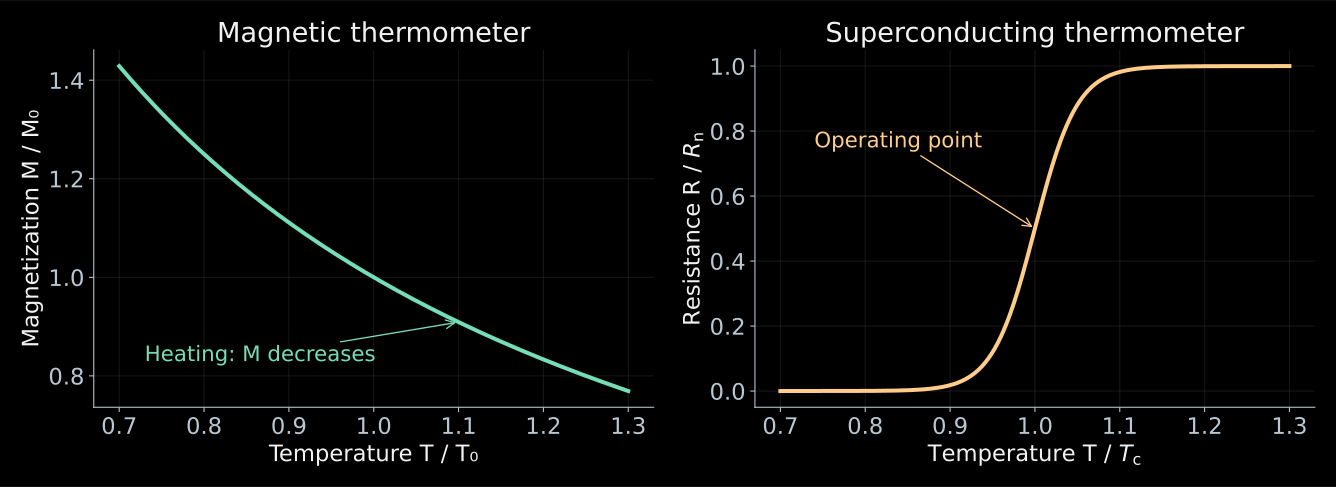
- The thermal signal is the same. What differs are the physical quantities with which the temperature is measured.
- The curves are schematic; for the magnetic sensor the weak-field Curie law is shown, for the TES a model of the transition.
Two decays can look like one
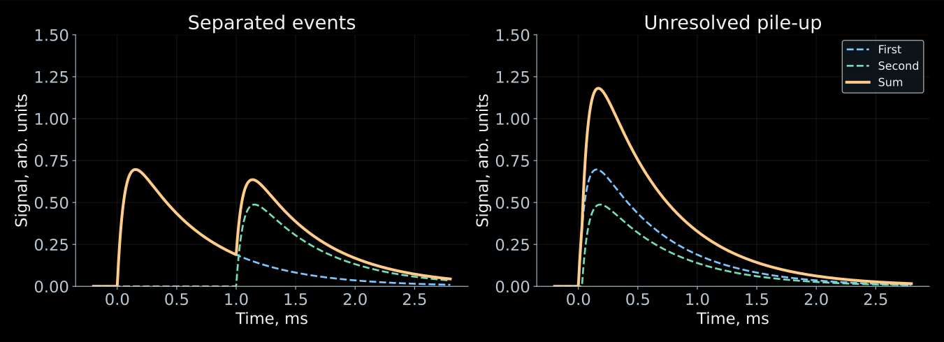
- If two events occur too close in time, the electronics can reconstruct one event with energy \(E_1+E_2\).
- Low-energy decays then land in the region of the end of the spectrum. The summed spectrum acquires events even above \(Q\).
- Let the activity of a single pixel be \(a\) decays per second, and let intervals shorter than \(\tau_r\) be unresolved.
- The probability of the next decay within this interval:
\[ \boxed{ f_{\mathrm{pu}}=1-e^{-a\tau_r} \simeq a\tau_r,\qquad a\tau_r\ll1 }. \]
- For \(a=10~\text{s}^{-1}\) and \(\tau_r=1\) μs we obtain \(f_{\mathrm{pu}}\sim10^{-5}\).
- This is a small fraction of all events, but there are even fewer useful events at the end of the spectrum.
- For independent decays the energy distribution of pile-up events is proportional to the convolution \(S*S\), where \(S(E_c)\) is the single-event spectrum.
- For \(N\) identical pixels and total activity \(A_{\mathrm{tot}}=Na\), the number of single decays grows as \(A_{\mathrm{tot}}\).
- The rate of close pairs in the whole array is approximately
\[ \boxed{ R_{\mathrm{pu}}\simeq Na^2\tau_r =\frac{A_{\mathrm{tot}}^2\tau_r}{N} }. \]
- For a fixed total activity, spreading it over a larger number of pixels reduces pile-up.
- Many channels must be read out and calibrated simultaneously. The channels can be distinguished by the individual frequencies of the resonators in a common readout line.
Missing momentum: pion and tau
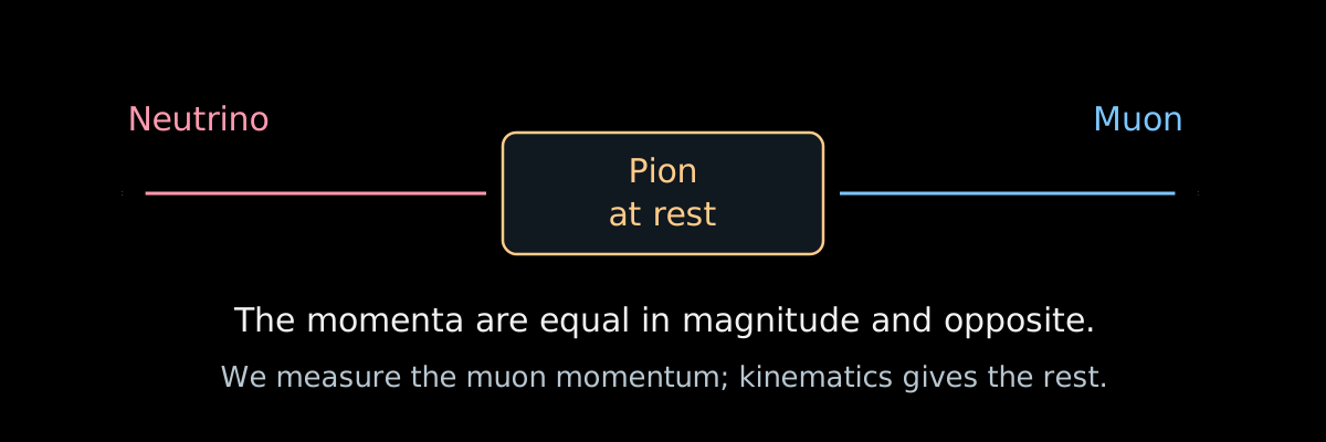
- In the decay \(\pi^+\to\mu^++\nu_\mu\), a pion at rest gives the muon and the neutrino momenta of equal magnitude. It suffices to measure \(p_\mu\):
\[ \boxed{ m_\nu^2=(P_\pi-P_\mu)^2 =m_\pi^2+m_\mu^2-2m_\pi\sqrt{p_\mu^2+m_\mu^2} }. \]
- For zero mass
\[ p_\mu=\frac{m_\pi^2-m_\mu^2}{2m_\pi}\simeq29.79~\text{MeV}. \]
- Measurement by Assamagan et al.: \(m_{\nu_\mu}<170\) keV (\(90\%\)).
Measurement of the muon momentum in pion decay. The notation \(m_{\nu_\mu}\) is traditional for this channel; the flavor state has no definite mass of its own.
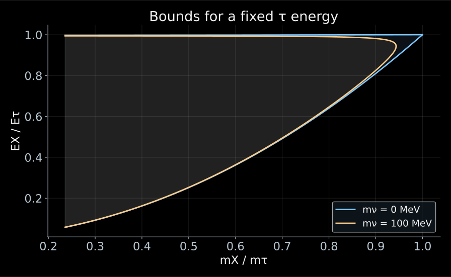
- In \(\tau^-\to X^-+\nu_\tau\), the four-momenta of the detected hadrons are added, giving the mass \(m_X\) and the energy \(E_X\) of the visible system.
- The neutrino mass cuts off the edge of the accessible region:
\[ m_X\le m_\tau-m_\nu. \]
- The tau is moving, so the boundary in energy is smeared into a band between \(\cos\theta^*=\pm1\). The mass is sought from how the events lie near the edge of the band.
- ALEPH: \(m_{\nu_\tau}<18.2\) MeV (\(95\%\)).
- In the figure, \(\gamma_\tau=10\) and the mass \(100\) MeV, so that the effect is visible.
- Let us differentiate the relation between the mass and the muon momentum:
\[ \delta m_\nu^2=-2m_\pi\frac{p_\mu}{E_\mu}\,\delta p_\mu. \]
- To be sensitive to \(m_\nu=1\) eV, the momentum of \(29.79\) MeV must be known with a relative precision of \(5\cdot10^{-16}\).
- Compare with tritium, where the limit is \(0.45\) eV: the pion channel is weaker by a factor of \(4\cdot10^5\), and the tau channel by a factor of \(4\cdot10^7\).
- The entire difference lies in the energy scale: tritium works with tens of keV, whereas here hundreds of MeV have to be subtracted.
Method four: record the arrival time
- For a mass state \(i\)
\[ v_i=c\sqrt{1-\frac{m_i^2c^4}{E_\nu^2}} \simeq c\left(1-\frac{m_i^2c^4}{2E_\nu^2}\right). \]
- Relative to a particle emitted simultaneously and moving with velocity \(c\),
\[ \boxed{ \Delta t_i=\frac{L}{v_i}-\frac{L}{c} \simeq\frac{L}{2c}\frac{m_i^2c^4}{E_\nu^2} }. \]
- A long baseline amplifies the delay; a high energy reduces it.
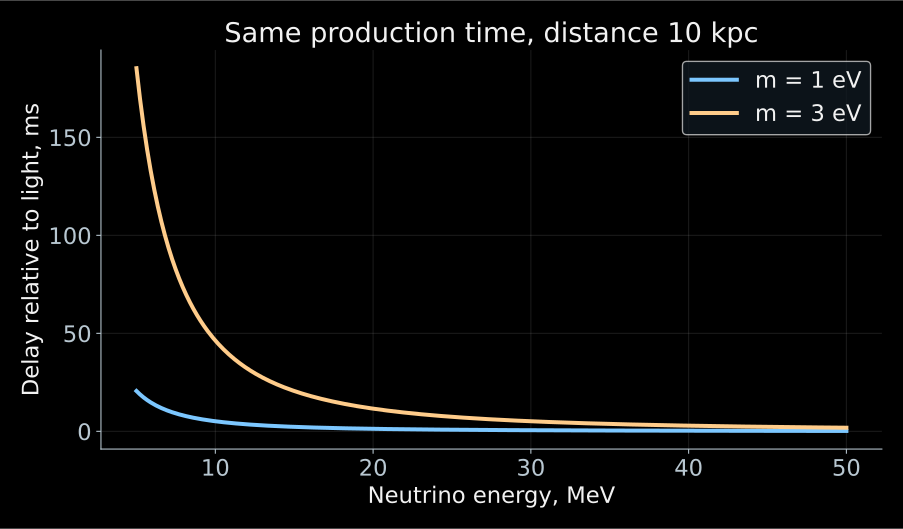
\[ \Delta t_i\simeq5.15~\text{ms} \left(\frac{L}{10~\text{kpc}}\right) \left(\frac{m_ic^2}{1~\text{eV}}\right)^2 \left(\frac{10~\text{MeV}}{E_\nu}\right)^2. \]
- Over tens of thousands of years of flight, a mass of order eV gives a delay of order milliseconds.
- The energy dependence \(1/E_\nu^2\) helps to search for this effect in a supernova signal.
- The detector measures the sum of three terms:
\[ t_{\mathrm{arr}} =t_{\mathrm{prod}}+\frac{L}{c}+\Delta t_i. \]
- The moment of the burst is unknown to us, and a shift of all times is absorbed by it without a trace. Only the energy dependence of the delay works.
- Moreover, a supernova emits neutrinos over several seconds, whereas the delay we are looking for is milliseconds.
- Therefore one needs either a model time profile of the source or a sufficiently sharp feature in the signal.
- A single quantity \(m_\beta^2\) is not enough here: the flux contains the mass states separately.
- In the coordinates \((1/E^2,\ t)\), the delay lies on a straight line, and its slope is \(m^2\).
- The slider for the spread of the emission time shows how quickly the signal is drowned out.
- On the right is the profile \(-2\ln L(m^2)\); its minimum is the mass estimate, and the width at the level \(+1\) gives the error.
Open the applet (in Russian) · the likelihood method is covered in my course on statistical analysis.
Why strive for tens of millielectronvolts?
- In tritium β decay and electron capture one measures
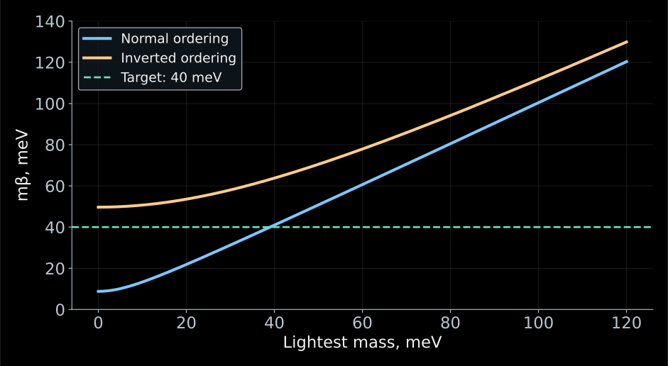
\[ m_\beta^2=\sum_i|V_{ei}|^2m_i^2. \]
- Oscillations fix the mass-squared differences and the mixing coefficients, but leave the lightest mass unknown.
- Even if the lightest mass is small, \(m_\beta\) does not vanish.
- The line \(40\) meV in the plot marks the target of a future experiment. There are as yet no constraints at this level.
- For normal ordering and \(m_1\simeq0\):
\[ m_\beta^2 \simeq |V_{e2}|^2\Delta m_{21}^2 +|V_{e3}|^2\Delta m_{31}^2. \]
- Let us substitute the rounded values \(|V_{e2}|^2\simeq0.30\), \(|V_{e3}|^2\simeq0.022\), \(\Delta m_{21}^2\simeq7.5\cdot10^{-5}\) eV\(^2\), \(|\Delta m_{31}^2|\simeq2.5\cdot10^{-3}\) eV\(^2\):
\[ m_\beta\simeq \sqrt{0.30\cdot7.5\cdot10^{-5}+0.022\cdot2.5\cdot10^{-3}} \simeq9~\text{meV}. \]
- For inverted ordering and \(m_3\simeq0\), almost the entire electron weight lies in two states with masses of about \(50\) meV; therefore \(m_\beta\simeq50\) meV.
| Measurement | Combination of masses | Additional physics |
|---|---|---|
| Electron kinematics | \(m_\beta^2=\sum_i|V_{ei}|^2m_i^2\) | decay spectrum and response |
| \(0\nu2\beta\) via light neutrinos | \(m_{\beta\beta}=|\sum_iV_{ei}^2m_i|\) | Majorana phases, nuclear amplitude |
| Cosmology | \(\Sigma=m_1+m_2+m_3\) | evolution of the Universe and the set of observations |
- In the β spectrum, the different unobservable mass states are added with their probabilities.
- In the Majorana amplitude, interference is possible. In cosmology, one measures the influence of neutrinos on the evolution of matter.
- Therefore these quantities cannot be compared as three measurements of the same number.