viewof katrinWindow = Inputs.range([1, 35], {
  value: 12,
  step: 1,
  label: html`
    <span class="spectrum-slider-label">
      ${tex`\Delta,\ \text{eV}`}
    </span>
  `
})

katrinResolution = 0.95
katrinMass = 0
katrinXMin = -40
katrinXMax = 2
katrinThreshold = -katrinWindow

katrinShape = x => {
  const neutrinoEnergy = -x
  if (neutrinoEnergy <= katrinMass) return 0
  return neutrinoEnergy * Math.sqrt(
    neutrinoEnergy * neutrinoEnergy - katrinMass * katrinMass
  )
}

katrinTransmission = x => {
  const excess = x - katrinThreshold
  if (excess <= 0) return 0
  if (excess >= katrinResolution) return 1
  return excess / katrinResolution
}

katrinX = Array.from({length: 701}, (_, i) =>
  katrinXMin + (katrinXMax - katrinXMin) * i / 700
)

katrinNorm = katrinShape(katrinXMin)
katrinData = katrinX.map(x => ({
  x,
  spectrum: katrinShape(x) / katrinNorm,
  accepted: katrinShape(x) * katrinTransmission(x) / katrinNorm
}))

katrinIntegral = (data => {
  let sum = 0
  for (let i = 1; i < data.length; i += 1) {
    const dx = data[i].x - data[i - 1].x
    sum += 0.5 * dx * (data[i].accepted + data[i - 1].accepted)
  }
  return sum
})(katrinData)

katrinPlot = Plot.plot({
  width: 1110,
  height: 300,
  marginTop: 18,
  marginRight: 25,
  marginBottom: 45,
  marginLeft: 72,
  style: {
    background: "#ffffff",
    color: "#111111",
    fontSize: "20px"
  },
  x: {
    axis: "bottom",
    label: null,
    domain: [katrinXMin, katrinXMax],
    ticks: 8,
    grid: true
  },
  y: {
    axis: "left",
    label: null,
    domain: [0, 1.05],
    ticks: 5,
    grid: true,
    tickFormat: value => value.toFixed(1)
  },
  marks: [
    Plot.areaY(katrinData, {
      x: "x",
      y: "accepted",
      fill: "#ffb347",
      fillOpacity: 0.55
    }),
    Plot.line(katrinData, {
      x: "x",
      y: "spectrum",
      stroke: "#4ea1ff",
      strokeWidth: 4
    }),
    Plot.line(katrinData, {
      x: "x",
      y: "accepted",
      stroke: "#ffb347",
      strokeWidth: 3
    }),
    Plot.ruleX([katrinThreshold], {
      stroke: "#ffb347",
      strokeDasharray: "7,5",
      strokeWidth: 2.5
    }),
    Plot.ruleX([katrinThreshold + katrinResolution], {
      stroke: "#777777",
      strokeDasharray: "4,5",
      strokeWidth: 2
    }),
    Plot.frame({stroke: "#111111"})
  ]
})

html`
<div class="spectrum-panel">
  <div class="spectrum-legend">
    <span>
      <i class="spectrum-swatch spectrum-swatch-massless"></i>
      ${tex`d\Gamma/dE`}
    </span>
    <span>
      <i class="spectrum-swatch spectrum-swatch-massive"></i>
      transmitted part
    </span>
    <span>${tex`\Delta E=0.95\ \text{eV}`}</span>
  </div>
  <div class="spectrum-plot-row">
    <div class="spectrum-y-label">
      ${tex`d\Gamma/dE\;(\text{arb. units})`}
    </div>
    <div class="spectrum-plot-host">${katrinPlot}</div>
  </div>
  <div class="spectrum-x-label">${tex`E-E_0\;(\text{eV})`}</div>
  <div class="spectrum-summary">
    <span>${tex`\Delta\equiv E_0-e|U|=${katrinWindow}\ \text{eV}`}</span>
    <span>${tex`R(U)-b\ \propto\ ${katrinIntegral.toFixed(3)}`}</span>
  </div>
</div>`Direct Determination of the Neutrino Mass.
The KATRIN Experiment
Introduction to Neutrino Physics
From the decay to a registered electron
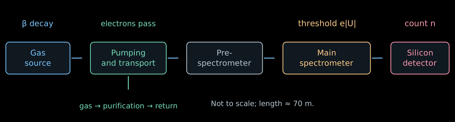
- Source: many decays in a gas of known composition.
- Transport: the electrons follow the magnetic field; the neutral gas is pumped out.
- Main spectrometer: each electron either passes or is reflected.
- Detector: during the time \(t\) the number of events \(n\) accumulates; the count rate is equal to \(R=n/t\).
Scheme: the main components of KATRIN.
Windowless source: the gas must flow
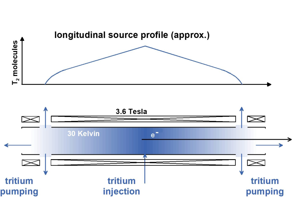
Scheme of the source: Drexlin, Weinheimer, fig. 6. WGTS is the windowless gaseous tritium source.
- Tritium is injected into the middle of a tube of length \(10\) m.
- Pumps at both ends continuously remove the gas. The density is maximal at the center and drops toward the exits.
- The gas is purified and returned to the source: a stationary flow is maintained.
- The electron does not pass through a film or a window. But other gas molecules remain on its path.
- The number of molecules per unit transverse area defines the column density:
\[ \rho d\equiv\int_0^d n(z)\,dz \simeq4\cdot10^{17}\ \mathrm{cm}^{-2}. \]
- \(n(z)\) is the concentration of molecules; \(\rho d\) is the accepted notation for the integral.
- The larger \(\rho d\), the more decays, but the more often the electron scatters. Therefore an instability of the density changes both the intensity and the shape of the spectrum.
- The injection pressure and the temperature \(T_{\mathrm{gas}}\) are stabilized: they determine the distribution of the gas. The thermal motion of the molecules also produces Doppler broadening of the spectrum.
It is important to know not only the number of decayed nuclei, but also the amount of gas that the electron will meet after being born.
- The gas contains \(\mathrm T_2\), \(\mathrm{DT}\), \(\mathrm{HT}\) and molecules without tritium. \(\mathrm T_2\) has two radioactive nuclei, \(\mathrm{DT}\) has one.
- Different molecules give different distributions of the final excitations of the daughter ion. This changes the production spectrum, as we saw in lecture 04.
- The composition is continuously measured by Raman spectroscopy: upon scattering, a laser photon gives the molecule energy of rotation or vibration,
\[ E_{\gamma,\mathrm{in}}-E_{\gamma,\mathrm{out}} =\Delta E_{\mathrm{mol}}. \]
- The positions of the lines distinguish the molecules, and their intensities, after calibration, give the concentrations of the components.
How many collisions will an electron experience?
- Let an electron be born at the point \(z\) and move toward the exit \(z=d\) at an angle \(\alpha\) to the axis of the almost uniform field. For the axial displacement \(dz'\) it travels the path \(dz'/\cos\alpha\). The mean number of inelastic collisions is equal to
\[ \boxed{ \tau(z,\alpha)= \frac{\sigma_{\mathrm{inel}}}{\cos\alpha} \int_z^d n(z')\,dz' }. \]
- This quantity is called the optical depth: the path expressed in mean free path lengths \(\lambda=1/(n\sigma_{\mathrm{inel}})\). In lecture 01 the ratio \(x/\lambda\) in the law \(P_0=e^{-x/\lambda}\) had the same meaning.
- For the whole column of gas
\[ \boxed{ \tau_{\mathrm{col}}=(\rho d)\,\sigma_{\mathrm{inel}} \simeq(4\cdot10^{17})(3.4\cdot10^{-18})\simeq1.36 }. \]
- The gun beam goes along the axis through the whole column, therefore \(\tau_{\mathrm{gun}}=\tau_{\mathrm{col}}\).
The angle and the cross section are assumed constant along the path. This is an approximation for estimating the probabilities; the change of direction in collisions is taken into account in a more complete model.
- The collisions are independent, therefore their number is Poisson distributed:
\[ \boxed{ P_n(z,\alpha)=e^{-\tau}\frac{\tau^n}{n!} }, \qquad \tau=\tau(z,\alpha). \]
- For the gun beam \(\tau=\tau_{\mathrm{col}}\simeq1.36\):
\[ P_0\simeq0.26, \qquad P_1\simeq0.35, \qquad P_2\simeq0.24, \qquad P_3\simeq0.11. \]
- At least one collision is experienced by three quarters of the beam, two or more by almost forty percent.
A single average correction for the lost energy will not do here: both the full distribution of losses and the weights of all multiplicities are needed.
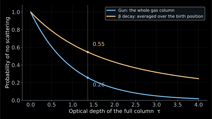
The numbers refer to different objects: \(0.26\) to the gun beam, \(0.55\) to the β electrons of the same gas. The gun measures the gas; to go over to the β spectrum one must average over the places of birth and the angles.
The probability of production is proportional to the concentration, therefore \(u\) is uniform for any shape of the profile \(n(z)\).
- The gun passes through the whole column, therefore the fraction of those that have not lost energy is equal to
\[ P_0^{\mathrm{gun}}=e^{-\tau_{\mathrm{col}}}\simeq0.26. \]
- The β electron is born inside the gas. For \(\alpha=0\) and constant composition the thickness remaining to the exit \(u\) is uniform on \([0,\tau_{\mathrm{col}}]\):
\[ \boxed{ \langle P_0\rangle_\beta =\frac{1}{\tau_{\mathrm{col}}}\int_0^{\tau_{\mathrm{col}}}e^{-u}\,du =\frac{1-e^{-\tau_{\mathrm{col}}}}{\tau_{\mathrm{col}}} \simeq0.55 }. \]
- Averaging over angles reduces this number: oblique trajectories are longer.
Electron gun: what do we measure?
Determine the energy-loss distribution in a single inelastic collision with a tritium molecule.
\(g_1(\varepsilon)\,d\varepsilon\) is the probability of a loss in the interval \([\varepsilon,\varepsilon+d\varepsilon]\) in such a collision.
\[ \int_0^\infty g_1(\varepsilon)\,d\varepsilon=1. \]
- \(g_1\) is the simplest object in this problem: a property of a single molecule, not of the apparatus. This function depends neither on the gas density, nor on the electron’s birth position, nor on the angle.
- Everything else is built from it: the losses in \(n\) collisions are convolutions \(g_1\), and the weights of the multiplicities are Poisson \(P_n(\tau)\).
Knowing \(g_1\) and \(\tau\), we know the loss distribution for any gas density and any path length in it.
For two independent collisions the losses add up: \(\varepsilon=\varepsilon_1+\varepsilon_2\).
\[ \boxed{ g_2(\varepsilon)= \int_0^\varepsilon g_1(x)\,g_1(\varepsilon-x)\,dx \equiv (g_1*g_1)(\varepsilon). } \]
The integral over all partitions of the total loss is a convolution.
For exactly \(n\) collisions:
\[ g_n=\underbrace{g_1*\cdots*g_1}_{n\ \text{times}}. \]
Convolution of distributions and the Poisson law are discussed in my course on statistical analysis.
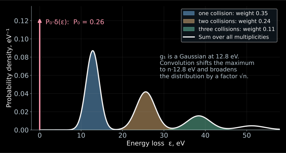
This is a teaching model, not a measured \(g_1\): the real function also has an ionization tail, which is visible in Fig. 11 at the end of this section.
- Toy model: \(g_1\) is a Gaussian centered at \(12.8\) eV with width \(1.6\) eV.
- The contribution of exactly \(n\) collisions is \(P_ng_n\): the maximum moves to \(n\cdot12.8\) eV, the width grows as \(\sqrt n\), and the weight falls off according to the Poisson law.
- The full loss distribution of the beam:
\[ \boxed{ G(\varepsilon)=P_0\,\delta(\varepsilon) +\sum_{n\ge1}P_n\,g_n(\varepsilon) }. \]
- The red arrow is the contribution of \(P_0\delta(\varepsilon)\): electrons without losses.
How are energy losses measured?
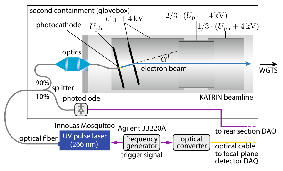
KATRIN, Fig. 2. The light is chosen close to the photoelectric threshold in order to reduce the initial energy spread.
Recall: \(\tau_{\mathrm{col}}=(\rho d)\sigma_{\mathrm{inel}}\simeq1.36\) is the optical depth of the entire column, \(P_n=e^{-\tau}\tau^n/n!\) is the probability of exactly \(n\) collisions, \(g_n\) is the distribution of the energy loss after them.
Ultraviolet light liberates electrons from the photocathode, and the electric field sets the energy \(E_{\mathrm{gun}}\simeq18.6\) keV. The beam passes through the entire gas column almost along the axis.
What matters is neither the energy nor the barrier separately, but their difference:
\[ \boxed{E_s=E_{\mathrm{gun}}-e|U|}. \]
\(E_s\) is the surplus energy (hence the subscript \(s\)). With a sharp filter, an electron passes if
\[ E_{\mathrm{gun}}-\varepsilon>e|U| \quad\Longleftrightarrow\quad \boxed{\varepsilon<E_s}. \]
In other words, \(E_s\) is the largest loss that the filter lets through. By scanning \(E_s\), we scan the threshold in losses.
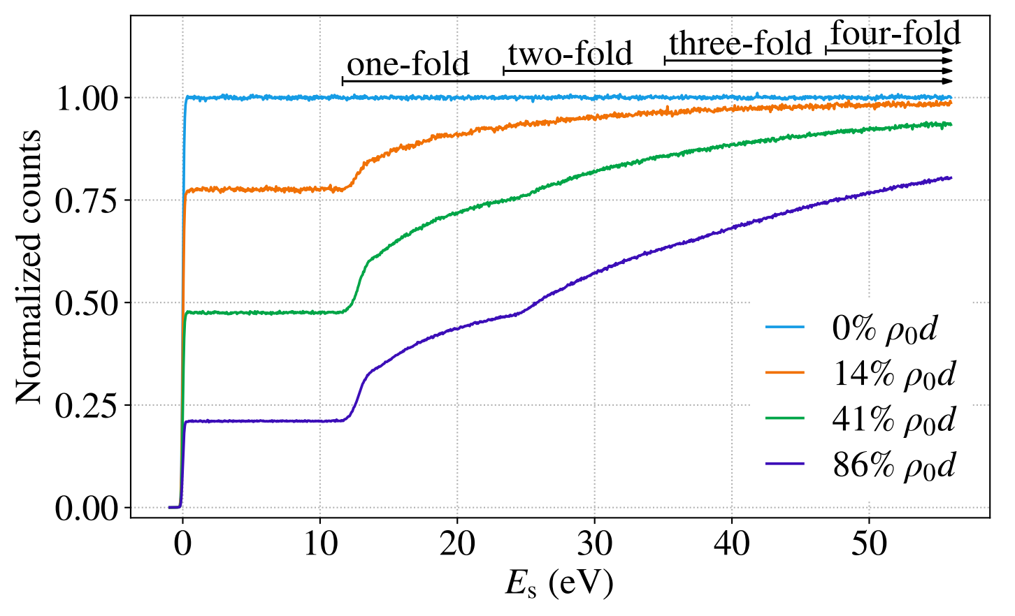
KATRIN, Fig. 3 shows the measured curves. The background and changes in the gun intensity are taken into account in the analysis.
- The horizontal axis is \(E_s\), the largest transmitted loss. The vertical axis is the normalized count \(r_{\mathrm{gun}}\): the ratio to the count without gas at large \(E_s\).
- No gas (light blue): a step at \(E_s=0\). Its width is the intrinsic resolution of the gun and the filter; this is the function \(\mathcal T_{\mathrm{gun}}(E_s)\).
KATRIN, Fig. 3 shows the measured curves. The background and changes in the gun intensity are taken into account in the analysis.
- Plateau: only electrons without losses have passed. As long as \(E_s\) has not grown to the smallest possible loss (\(\simeq11\) eV), there is nothing to add:
\[ r_{\mathrm{gun}}^{\text{plateau}}\simeq P_0=e^{-\tau}. \]
- Rise: at \(E_s\simeq12\) eV the singly scattered electrons pass, at \(\simeq25\) the doubly scattered ones, at \(\simeq37\) the triply scattered ones.
KATRIN, Fig. 3 shows the measured curves. The background and changes in the gun intensity are taken into account in the analysis.
- The plateau tells us how many electrons lost nothing: the heights \(0.78\), \(0.48\), \(0.21\) at \(14\), \(41\), \(86\,\%\) of \(\rho_0d\) give \(\tau=-\ln P_0\simeq0.25\), \(0.73\), \(1.56\).
- The rise tells us how the others lose energy: its shape follows the integral of \(g_1\).
- The denser the gas, the lower the plateau and the more pronounced the multiple collisions.
- The shape of \(g_1\) does not change in the process — this is what the separation of parameters rests on. \(\mathcal T_{\mathrm{gun}}\) refers to the nearly axial beam of the gun.
- The transmission for isotropic β electrons will be constructed before we assemble the response function.
Reconstructing the loss function
Recall the notation of the previous two slides: \(P_n\) is the probability of \(n\) collisions, \(g_n\) is the distribution of the total energy loss after them, \(\mathcal T_{\mathrm{gun}}(E_s)\) is the measured transmission of the gun without gas.
A loss \(\varepsilon\) shifts the argument of the transmission: \(\mathcal T_{\mathrm{gun}}(E_s-\varepsilon)\). We average over the losses after \(n\) collisions:
\[ (\mathcal T_{\mathrm{gun}}*g_n)(E_s) = \int_0^\infty g_n(\varepsilon)\, \mathcal T_{\mathrm{gun}}(E_s-\varepsilon)\,d\varepsilon. \]
We sum the contributions with the probabilities \(P_n\):
\[ \boxed{ \begin{aligned} r_{\mathrm{gun}}(E_s) &=P_0\,\mathcal T_{\mathrm{gun}}(E_s) +P_1(\mathcal T_{\mathrm{gun}}*g_1)(E_s)\\ &\quad+P_2(\mathcal T_{\mathrm{gun}}*g_2)(E_s)+\ldots \end{aligned} } \]
\(r_{\mathrm{gun}}\) is the normalized gun signal; the background is taken into account separately. KATRIN, equations (6)–(9).
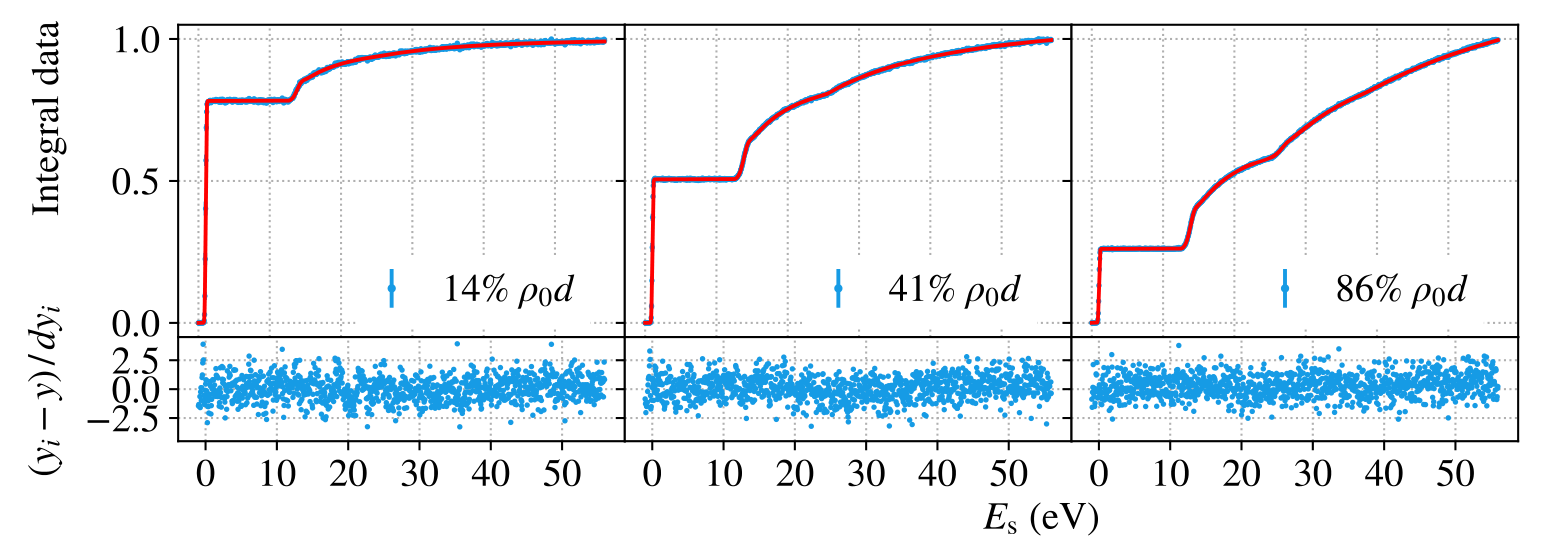
KATRIN, Fig. 10, top row shows the same measurements as in Fig. 3, but now together with the model. Fig. 3 shows the curves themselves: all densities on one panel, normalized to the count without gas. Fig. 10 shows the result of the joint fit: data, model, and residuals, with each panel normalized to its own last bin — so the plateau height here is no longer equal to \(P_0\). The joint fit also includes the differential time-of-flight data.
Why different densities separate the parameters: \(\tau\) shifts the height of the plateau and the weights of the steps, while \(g_1\) sets their shape. By varying \(\rho d\), we mix these contributions in different ways — and “how many collisions” is separated from “how a single collision loses energy”.
- Common to all data sets: the shape of \(g_1\). Below the ionization threshold it is taken as a sum of three Gaussians, above it as a calculated ionization tail.
- Specific to each data set: the optical depth \(\tau\), the normalization, and the background.
- The parameters are fitted to all densities simultaneously: one and the same \(g_1\) must describe both the plateau height and the shape of all the steps.
- The lower panels show the normalized residuals \((y_i-y)/dy_i\). A scatter around zero without visible structure means that the fit succeeded.
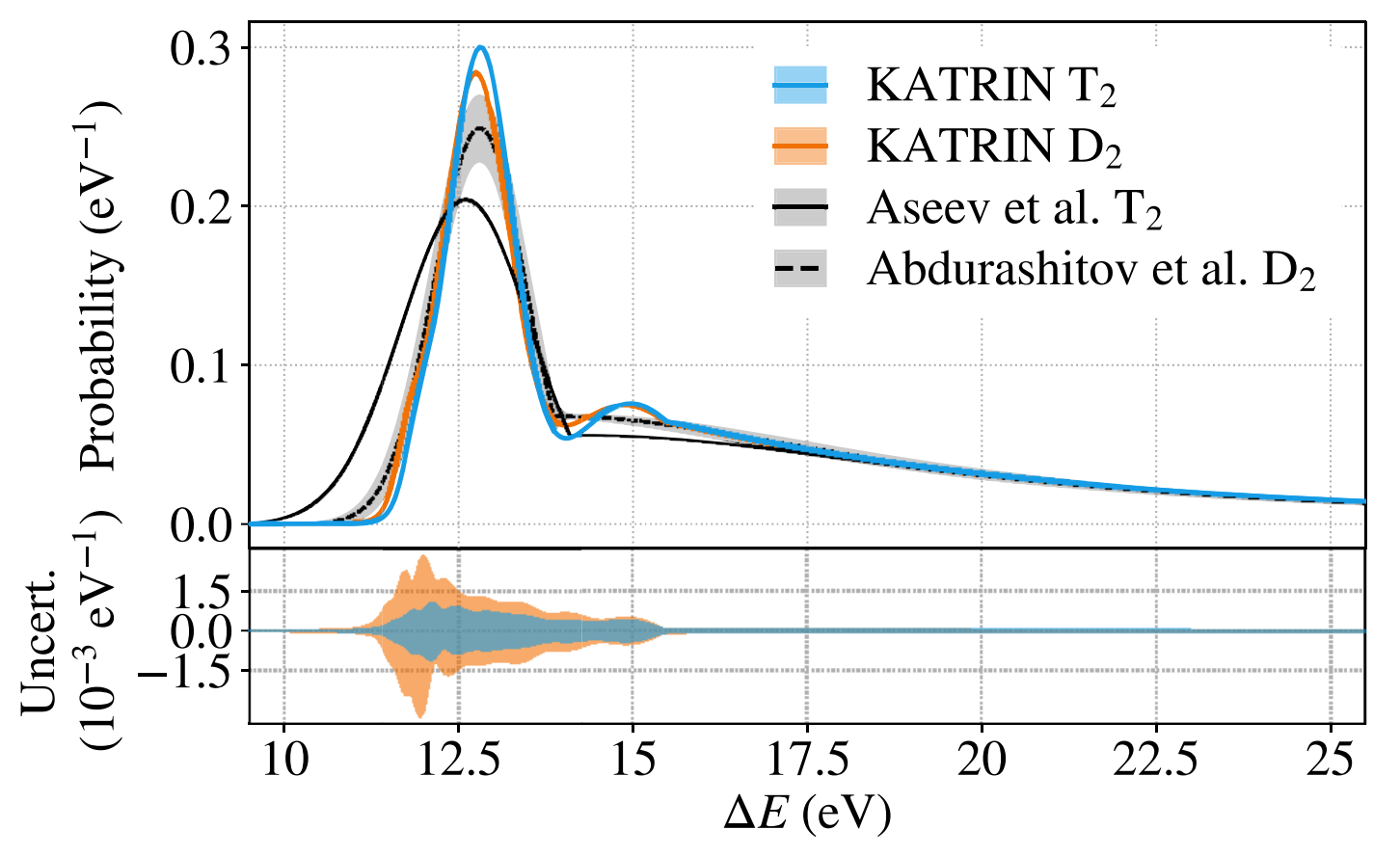
The light-blue curve is the \(g_1\) found for tritium.
The peak near \(12.8\) eV corresponds to electronic excitations of the molecule. The tail above \(15.5\) eV is ionization.
Next we use \(g_n\) in the calculation of the response of the β source, taking into account the birth positions and angles of the electrons.
KATRIN, Fig. 11. The horizontal axis shows \(\Delta E=\varepsilon\); the vertical axis shows the probability density, eV\(^{-1}\).
How to measure 18,600 volts to hundredths of a volt?
- A negative voltage \(U\simeq-18.6\) kV is applied to the vessel of the main spectrometer. A commercial source sets the main level, but its stability of order \(10^{-4}\) means fluctuations of about \(1\) V.
- A parallel post-regulator based on a vacuum triode picks a small correcting current and suppresses fast voltage fluctuations.
- The alternating component is measured by a ripple probe: it sees noise in the range up to about \(1\) MHz.
- The DC component is measured slowly, but precisely:
\[ U_{\rm vessel} \xrightarrow{\ \text{divider }M\simeq1972\ } u\simeq-9.4~\text{V} \xrightarrow{\ \text{voltmeter}\ } U_{\rm vessel}=Mu. \]
- The requirement \(3\cdot 10^{-6}\) at \(18.6\) kV means \(|\delta U|\lesssim56\) mV. For an electron this is a threshold shift of \(|\delta E|=e|\delta U|\lesssim56\) meV.
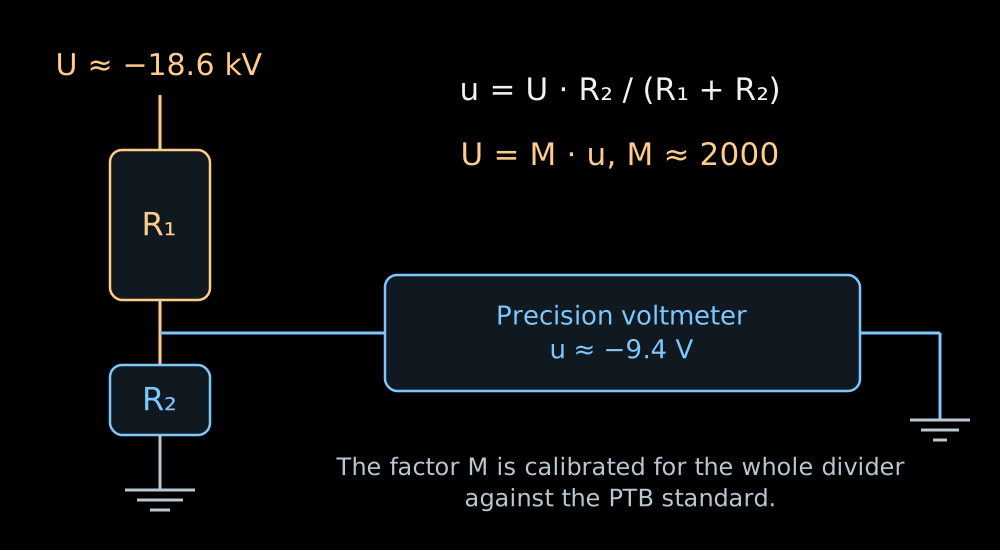
- The calculation uses the scale factor of the entire instrument, measured relative to the PTB reference divider:
\[ M(-18.6~\text{kV})=1972.4801\pm0.0040 \qquad (\text{expanded uncertainty},~k=2). \]
- In the K35 divider the high-voltage arm is a chain of one hundred resistors of \(1.84\) MΩ each. Each of them carries about \(186\) V and \(19\) mW.
- The low-voltage arm has a resistance of about \(93\) kΩ. The division ratio of the whole chain is
\[ M\equiv\frac{U}{u} =\frac{R_{\rm HV}+R_{\rm LV}}{R_{\rm LV}}, \qquad \boxed{U=Mu}. \]
- At \(|U|=18.6\) kV the voltmeter reads \(|u|\simeq9.43\) V. Such a signal is convenient to measure on the most accurate range of the voltmeter.
Krypton provides lines of known energy
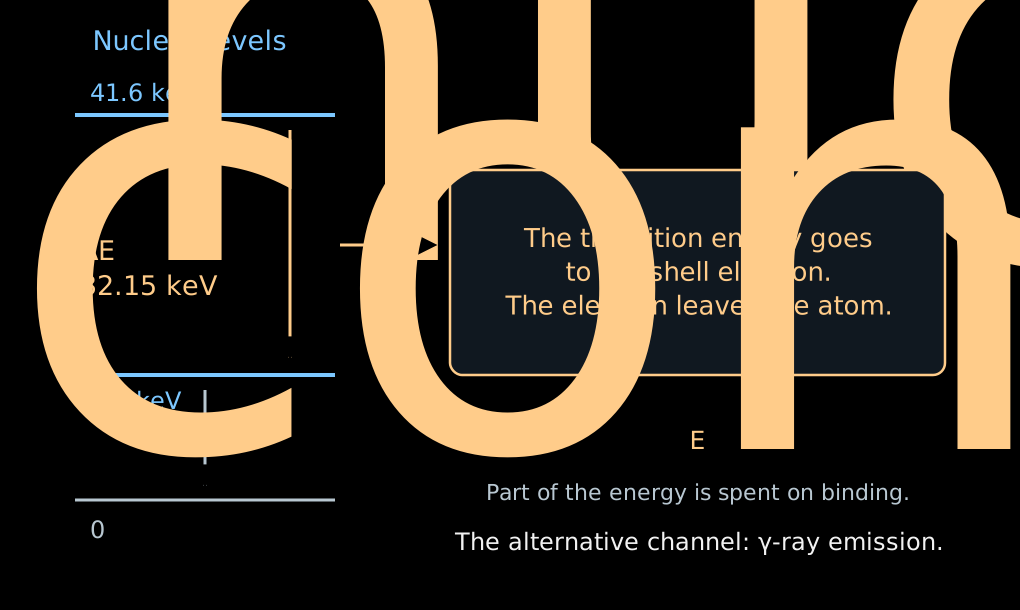
- An excited nucleus can transfer its energy directly to one of the electrons of the atomic shell. This is internal conversion.
- The electron leaves the atom; part of the transition energy is spent on its binding.
- For the shell \(a\):
\[ \boxed{ E_{\mathrm{conv},a} =\Delta E_{\mathrm{nucl}} -E_{\mathrm{bind},a} -E_{\mathrm{recoil}} }. \]
- There is no neutrino here carrying away a variable fraction of the energy. A fixed transition and a shell give a spectral line.
- The index \(\mathrm m\) denotes a metastable, long-lived excited state of the nucleus.
- In \(^{83\mathrm m}\mathrm{Kr}\), a transition with an energy of about \(32.15\) keV gives a conversion line of the \(K\) shell at about \(17.82\) keV — close to the end of the tritium spectrum.
- \(K\) is the electron shell closest to the nucleus; the line designation \(K\)-32 indicates the shell and the energy of the nuclear transition.
- The line has a natural width, about \(2.7\) eV for \(K\)-32. With a large number of electrons, the position of its center can be determined much more precisely than the width.
- For other tasks, narrower lines of other shells are used.
- We scan the retarding voltage across the line. The integral count rate changes from full transmission to zero.
- The position of the edge checks the energy scale.
- The shape of the edge depends on the natural width of the line, the spread of initial potentials, and the transmission of the spectrometer.
- Knowing the intrinsic shape of the line, one can determine additional shifts and broadenings of the apparatus.
- Lines of different shells allow the scale to be checked at several points. When the difference of their energies is used, the energy of the common nuclear transition cancels.
Monitor spectrometer: checking the scale
- A small separate MAC-E spectrometer measures the conversion line of a stable \(^{83}\mathrm{Rb}/{}^{83\mathrm m}\mathrm{Kr}\) source.
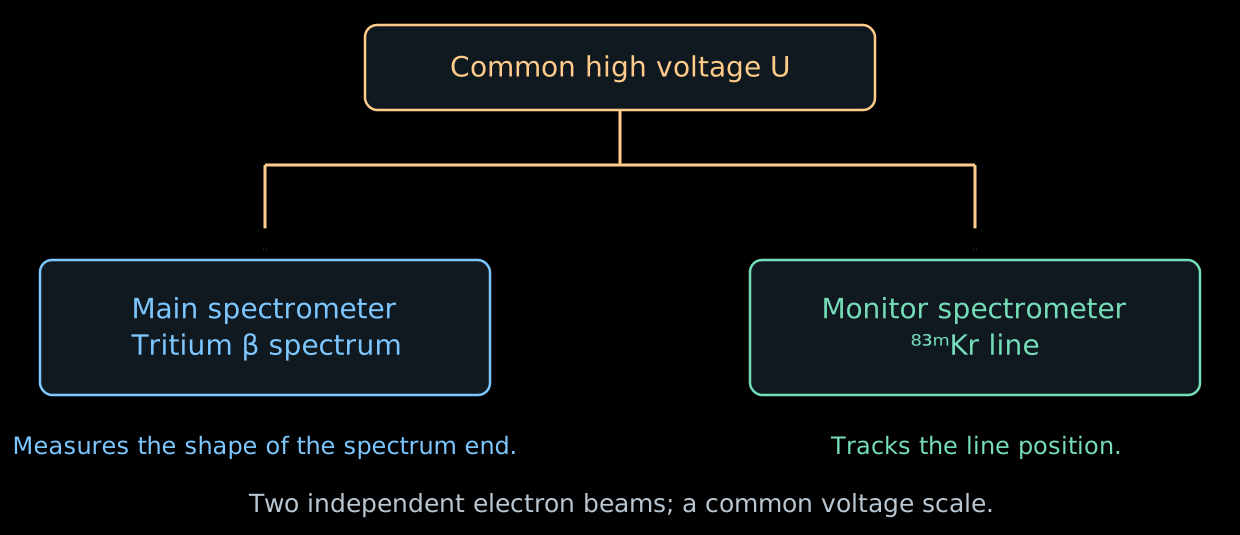
- It is connected to the same high voltage as the main spectrometer. The \(K\)-32 line lies about \(0.8\) keV below the endpoint of the tritium spectrum; a separate voltage on the source shifts it to the required working region.
- If the line has shifted while the source is stable, the energy scale has changed. This can be compared with the readings of the voltage divider.
- The monitor checks the stability of the scale over time. The gaseous source and local inhomogeneities of the main spectrometer require their own calibrations.
The background changes the design of the experiment
- In Lecture 06, the magnetic mirror held particles in a trap. In the spectrometer, it can trap an electron of radioactive origin.
- The electron repeatedly passes through the residual gas and produces secondary electrons by ionization. A single primary decay can give a series of counts.
- Therefore the background count can have a larger variance than an independent Poisson flux.
- Radon from the materials is held back by cold traps in the pumping ports. Electrons from the walls are suppressed by the magnetic configuration and by a more negative potential of the wire electrodes.
- The pre-spectrometer was originally intended to reflect in advance electrons with energies far below the endpoint of the β spectrum.
- But a confinement region arose between the two electrostatic barriers: along the axis the electric fields prevented escape, and transversely the magnetic field did. This is a Penning trap.
- The accumulation of charged particles led to a background growing with time.
- For later campaigns, the retarding voltage of the pre-spectrometer was reduced to the order of \(100\) V. The main spectrometer continued to set the precise energy threshold.
An additional filter is useful as long as it does not itself become a source of counts.
- Part of the background is born from neutral excited atoms entering the volume from the walls.
- A weakly bound electron can be freed even by the thermal radiation of the walls.
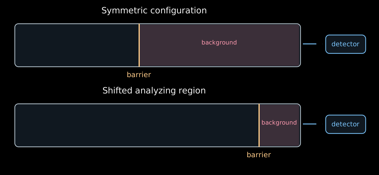
- If the barrier is shifted toward the exit and the magnetic flux tube is compressed, the volume available to the background after the barrier decreases.
- This configuration reduced the background by about a factor of two. The inhomogeneous fields in it are calibrated with krypton.
The available volume is shown schematically; the geometry of the field lines is omitted. KATRIN shifted analyzing region.
- The teaching example of Lecture 06 used a symmetric configuration:
\[ B_{\mathrm{src}}=3.6~\mathrm{T},\quad B_{\mathrm A}=0.30~\mathrm{mT},\quad B_{\max}=6.0~\mathrm{T} \quad\Rightarrow\quad \Delta E\simeq0.95~\mathrm{eV}. \]
- For the characteristic fields of the shifted configuration
\[ B_{\mathrm{src}}\simeq2.5~\mathrm{T},\quad B_{\mathrm A}\simeq0.6~\mathrm{mT},\quad B_{\max}\simeq4.2~\mathrm{T} \quad\Rightarrow\quad \Delta E\simeq2.7~\mathrm{eV}. \]
- For larger \(B_{\mathrm A}\), the magnetic flux tube is narrower and the transmission edge is wider.
- The loss of resolution is weighed against the gain from the lower background. The parameters are chosen according to the final uncertainty of \(m_\beta^2\).
- In the real shifted region, \(B_{\mathrm A}\) and the potential depend on position; a single number here gives only a characteristic scale.
Where is the mass in the integral spectrum?
- To see the dependence on the mass, we temporarily keep a single final state, an ideal sharp filter, and a constant slowly varying factor \(C\).
- Introduce \(x=E_0-E\) and \(w=E_0-e|U|\). The quantity \(w\) is the width of the energy window between the threshold and the endpoint of the spectrum. For \(w>m_\beta\):
\[ R(w)-b =AC\int_{m_\beta}^{w}x\sqrt{x^2-m_\beta^2}\,dx =\boxed{\frac{AC}{3}(w^2-m_\beta^2)^{3/2}}. \]
- For \(w\gg m_\beta\) the expansion gives
\[ \boxed{ R(w)\simeq AC\left(\frac{w^3}{3}-\frac{m_\beta^2w}{2}\right)+b }. \]
- The massless signal grows as \(w^3\); the mass adds a deficit proportional to \(m_\beta^2w\).
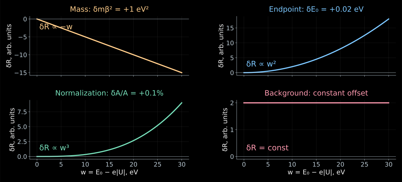
Linearized model of the previous tab. The changes in the count rate are shown with all other parameters held fixed; the vertical axis scales are different.
- At a single point, a deficit of counts can be explained by the mass, by a lower activity, or by a shift of the energy threshold.
- At several points these explanations give different dependences:
\[ \frac{\partial R}{\partial m_\beta^2}\simeq-\frac{AC}{2}w,\quad \frac{\partial R}{\partial E_0}\simeq ACw^2,\quad \frac{\partial R}{\partial A}\simeq\frac{C}{3}w^3,\quad \frac{\partial R}{\partial b}=1. \]
- When differentiating with respect to \(E_0\), the voltage \(U\) is fixed: \(w=E_0-e|U|\) changes.
- The shape of the scan makes it possible to separate the four parameters, although their estimates remain correlated.