Neutrino Telescopes

Principles, Results, and Prospects

Dmitry Naumov

A new window on the Universe

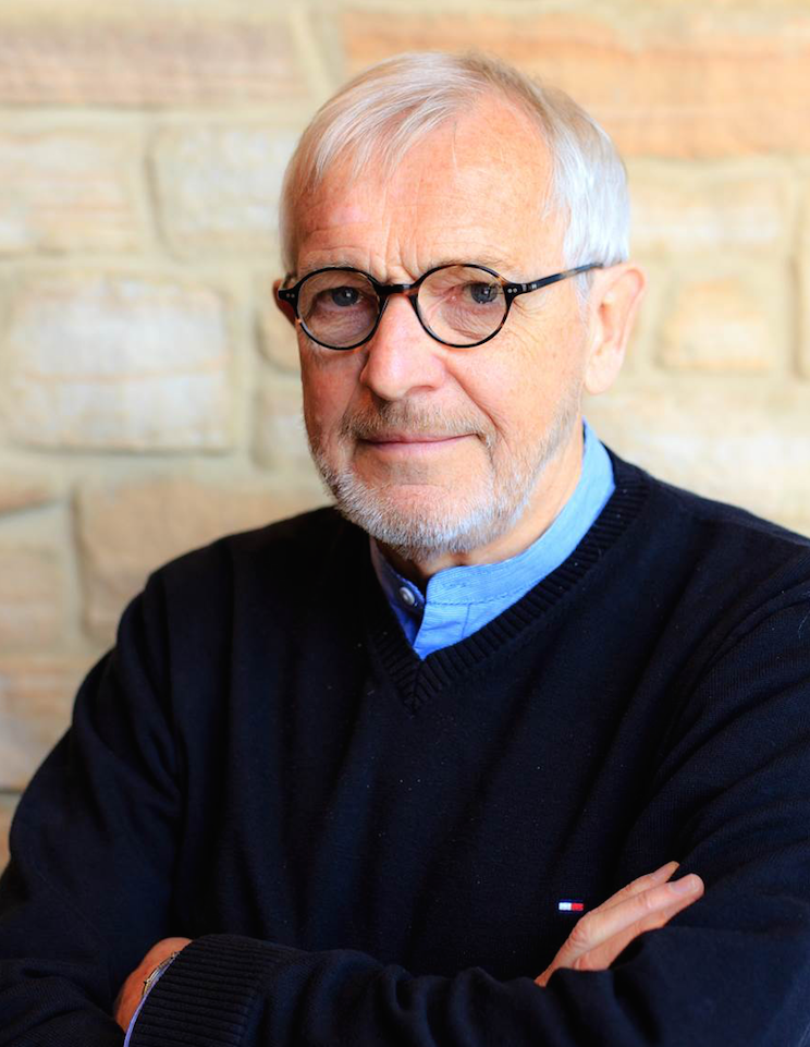
Francis Halzen.

Francis Halzen.

2026 Nobel Prize in Physics

IceCube and the discovery of high-energy astrophysical neutrinos.

\(1\,\mathrm{PeV} = 10^{15}\,\mathrm{eV}\)

in a single neutrino

a billion times a neutrino from the Sun

over a hundred times a proton in the LHC

Not nuclear fusion. Then what? And where?

Sensor positions: IceCube geometry · light pattern modelled · Bert and Ernie: IceCube 2013 · Big Bird: IceCube 2014, position illustrative

History of Neutrino Telescopes

A telescope inside a natural medium

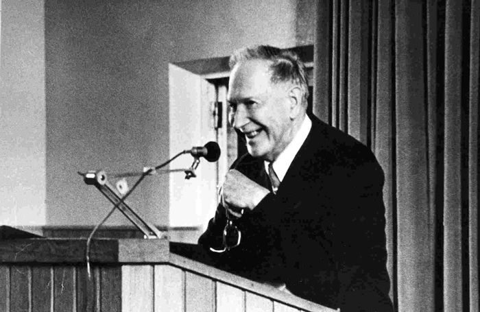
Moisei Markov speaking at a lectern.

Moisei Markov.

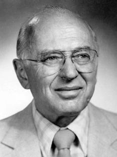
Kenneth Greisen, portrait reproduced in Spiering's historical review.

Kenneth Greisen. Undated portrait via C. Spiering.

1960: Markov and Greisen, independently. A large target already exists in nature.

  • Place light sensors deep in a lake or sea.
  • Use Cherenkov light to reconstruct charged particles produced by neutrinos.

M. A. Markov, Rochester conference, 1960, p. 578.

From DUMAND to the first working telescopes
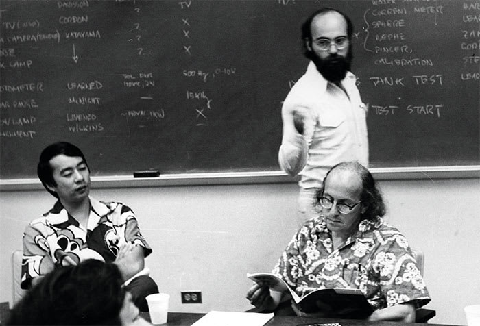
John Learned at the blackboard, Jed Hirota seated at left and Dick Davisson seated at right, DUMAND 1976 workshop.

DUMAND workshop, 1976. John Learned at the board; Jed Hirota (left), Dick Davisson (right). Photo: Anatoly Petrukhin, via IceCube.

DUMAND, near Hawaii: the first deep-ocean attempt

  • 1993: the first string on the sea floor sees muons. Seawater seeps in and a short circuit ends the test.
  • 1995: support ends. The array is never built.

Other routes kept going

  • Baikal: NT36, three strings and 36 optical modules, 1993.
  • AMANDA: polar ice.
  • ANTARES: the Mediterranean; the 12-line detector is complete in 2008.

“Congratulations for winning the 3-string race!”

Francis Halzen to Christian Spiering

NT36, DUMAND’s TRIAD and AMANDA: competing routes to a working array.

DUMAND Collaboration, astro-ph/9412019; C. Spiering, Eur. Phys. J. H 37, 515 (2012), arXiv:1207.4952.

The method works: the road to IceCube

1996Baikal NT96: a clear upward-going neutrino signal 1998Baikal NT200 completed with 192 optical modules 1990sAMANDA: deeper ice makes directional reconstruction possible 1999The AMANDA team proposes a cubic-kilometre detector, IceCube thenFunding for construction is granted 2004–05First IceCube construction season 2010The last of 86 strings 2013An astrophysical neutrino flux

Atmospheric neutrinos showed that Markov’s method works, in a lake and in ice.
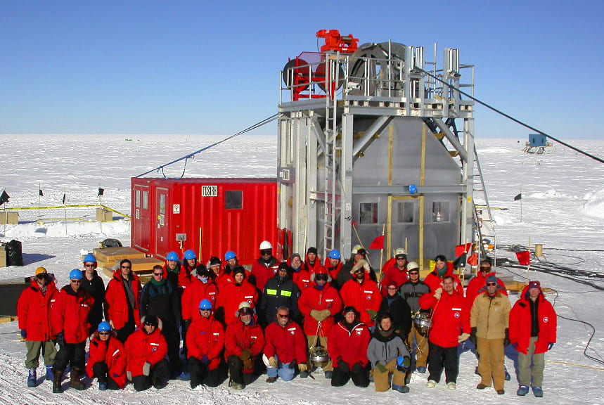
The IceCube construction team in the 2004–2005 season, in front of a drilling tower.

First IceCube construction season, 2004–2005. IceCube/NSF historical archive.

C. Spiering, historical review (2024), slides 29–31; Baikal detector paper; IceCube timeline.

Detection Principles

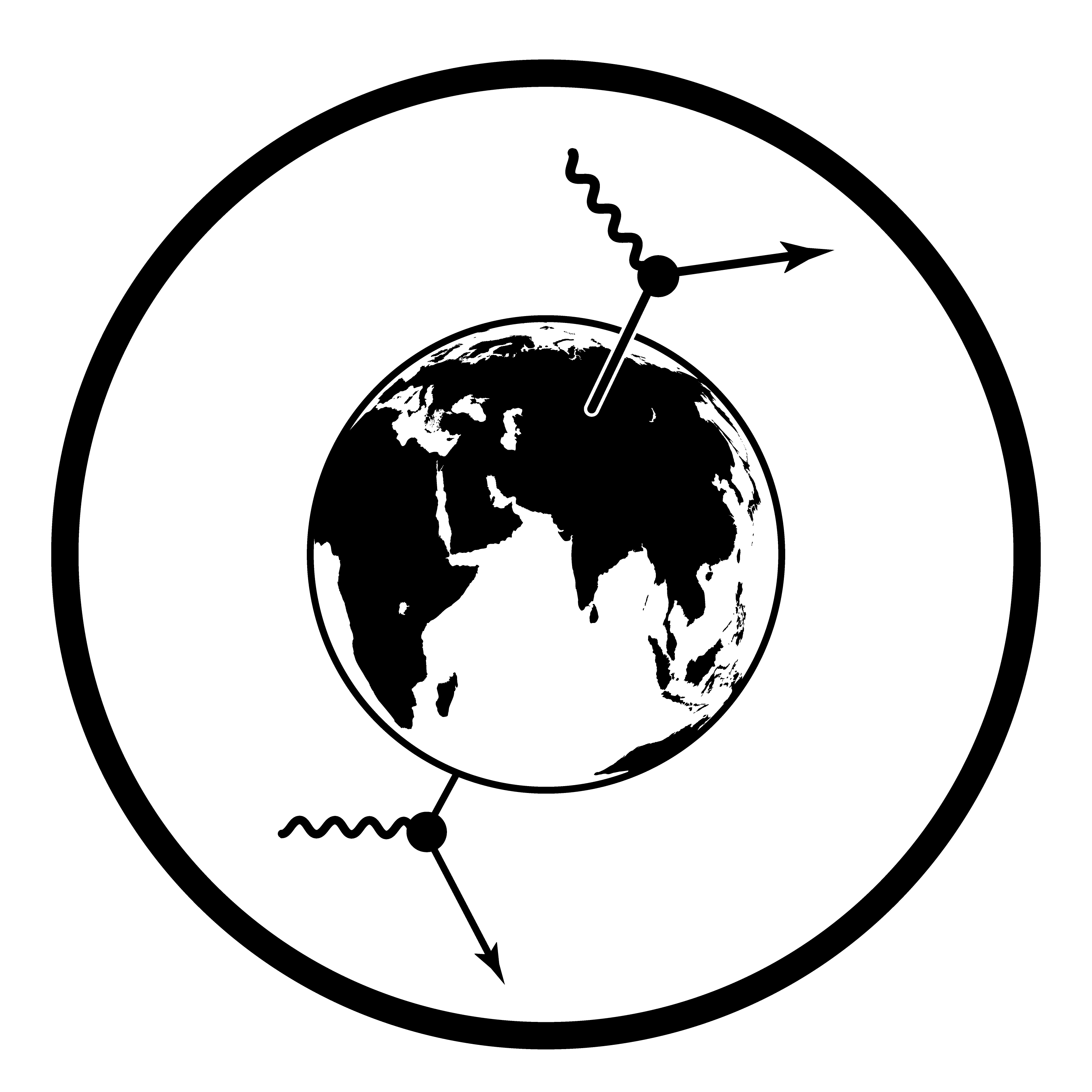
Transparent Universe, opaque Earth

A \(1\,\mathrm{PeV}\) muon neutrino in today’s mean baryonic matter

\[ \bar n_{b,0}\simeq0.25\,\mathrm{m^{-3}} =2.5\times10^{-7}\,\mathrm{cm^{-3}} \]

\[ \sigma_{\nu N}^{\mathrm{CC+NC}} \simeq9.5\times10^{-34}\,\mathrm{cm^2} \]

About one nucleon per four cubic metres.

\[ \lambda_{\nu N,0}=\frac{1}{\bar n_{b,0}\sigma_{\nu N}} \simeq4.2\times10^{39}\,\mathrm{cm} \]

\[ \lambda_{\nu N,0}\simeq4.4\times10^{21}\,\mathrm{ly} \]

Observable diameter today: \(D_{\rm obs}\simeq93\times10^9\,\mathrm{ly}\).

\[ \frac{\lambda_{\nu N,0}}{D_{\rm obs}}\simeq5\times10^{10} \]

Present-epoch \(\nu N\) estimate ignoring the Universe evolution. PDG baryon density; CSMS cross sections, Table I.
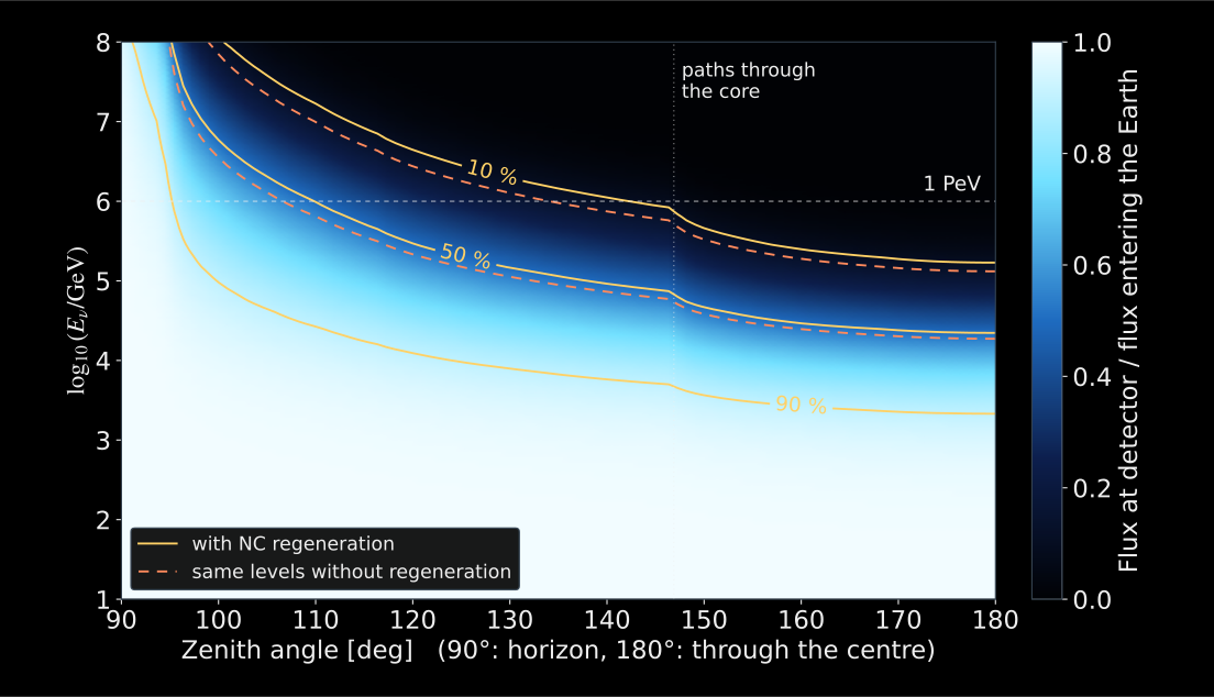
Ratio of the neutrino flux reaching a detector 1 km deep to the flux entering the Earth, versus zenith angle from 90 to 180 degrees and energy from 10 GeV to 100 PeV, with neutral-current regeneration. Near the horizon the Earth is transparent at all energies; through the centre half of the flux survives up to about 20 TeV and 10 percent up to about 170 TeV. Dashed contours without regeneration lie slightly lower in energy.

Full transport: V. A. Allakhverdyan (CT10nlo, PREM, detector 1 km deep), redrawn · V. A. Allakhverdyan, dissertation (2026), Fig. 4.20 · Allakhverdyan, Zavyalov & Naumov (2026), Fig. 9

\[ 1\,\mathrm{PeV}=10^6\,\mathrm{GeV} \]

Horizontal axis: zenith angle.

\(90^\circ\): near the horizon.

\(180^\circ\): through Earth’s centre.

Colour: flux at the detector over flux entering the Earth.

Dashed: without regeneration,

\[ e^{-N_A\,\sigma_{\rm tot}(E)\,X(\theta)}. \]

Neutral currents do not remove a neutrino; they move it to lower energy. With regeneration the ratio depends on the incident spectrum.

Tracks and cascades

Muon-neutrino interaction, 1 TeV · NTSim/Geant4 secondaries, LightHit radiative transfer in water · glow = expected photoelectrons, colour = first-light time · not sampled hits, not observed data · light front illustrative

Electron-neutrino interaction, 100 GeV · NTSim/Geant4 secondaries, LightHit radiative transfer in water · glow = expected photoelectrons, colour = first-light time · not sampled hits, not observed data · light front illustrative

Measured PMT signals; reconstructed track; illustrative cone. © KM3NeT. Official event display.
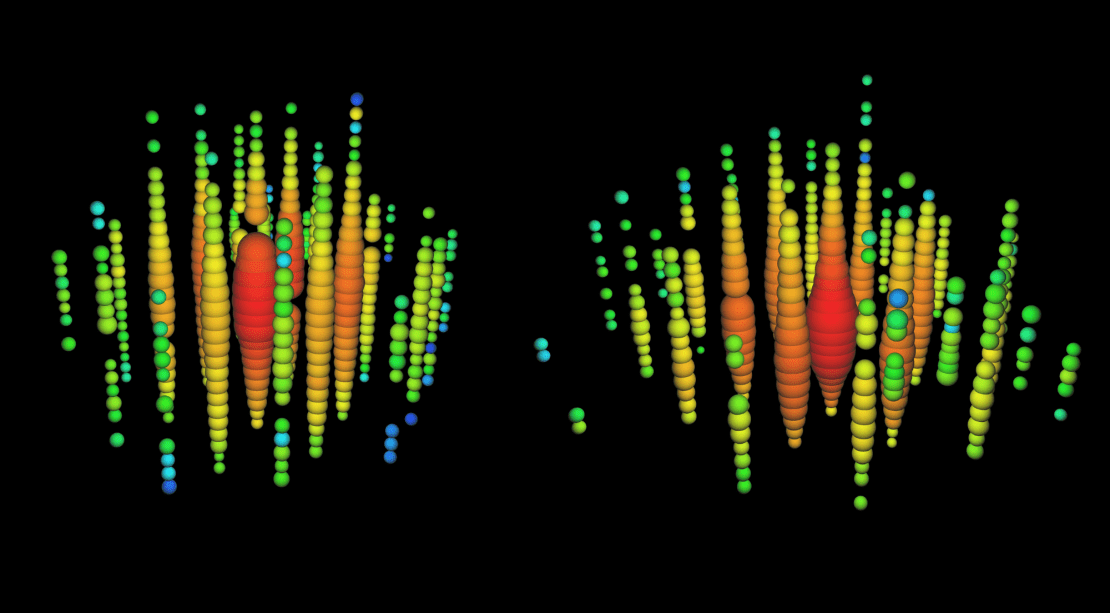
IceCube event displays of Bert and Ernie: hundreds of optical modules lit by two PeV cascades.

Bert and Ernie, the first PeV cascades: deposited energies \(1.04\pm0.16\) and \(1.14\pm0.17\,\mathrm{PeV}\). IceCube Collaboration / IceCube–NSF · IceCube (2013)

Cosmic Sources

Where jets get their power

  • Gas feeds an accretion disc around a supermassive black hole.
  • Magnetic fields can extract rotational energy and carry it into a jet.
  • The gas supply can sustain activity beyond a single stellar disruption.
  • Blazars: the jet points close to our line of sight.
  • Charged cosmic rays bend in magnetic fields.
  • Photons can scatter or be absorbed.
  • Neutrinos can escape dense environments and preserve directional information.

How jets produce neutrinos

Accelerated protons collide with nuclei in dense gas.

\[ pp\longrightarrow\pi^{\pm},\,\pi^0+X \]

Possible targets: a stripped stellar envelope or a gas cloud in the jet.

The gas density and the proton residence time control the interaction yield.

Accelerated protons interact with a radiation field.

\[ p\gamma\longrightarrow\pi^{\pm},\,\pi^0+X \]

Possible targets: synchrotron photons in the jet, or photons from the accretion disc and its surroundings.

The pion-production threshold depends on photon energy and collision angle.

Neutrinos from pion decay

\[pp\ \text{or}\ p\gamma\ \longrightarrow\pi^\pm,\,\pi^0+X\]

Charged pion and muon

\[ \begin{aligned} \pi^+&\to\mu^++\nu_\mu\\[0.5em] \mu^+&\to e^++\nu_e+\bar\nu_\mu \end{aligned} \]

Neutral pion

\[\pi^0\to\gamma+\gamma\]

Neutrinos and photons share the pion-production energy budget.

Charge-conjugate chain for \(\pi^-\) · Ahlers & Halzen (2018)

\[pp:\quad N_{\pi^+}:N_{\pi^-}:N_{\pi^0}\simeq1:1:1\]

\[ E_\nu^2\Phi_\nu(E_\nu)\simeq\frac32 E_\gamma^2\Phi_\gamma(E_\gamma), \qquad E_\gamma\simeq2E_\nu \]

At production: \(pp\) benchmark, all neutrino flavours and both signs.

Photon absorption and cascading modify the comparison with observed spectra.

Three messengers, one energy budget

Neutrinos and photons share the pion-production energy budget.

Conversion: Ahlers & Murase (2014) · absorption computed with the EBL of Domínguez et al. (2011) and the CMB · cascade shape schematic, energy conserved · Murase, Ahlers & Lacki (2013), Murase, Guetta & Ahlers (2016)

Observations

The astrophysical neutrino flux

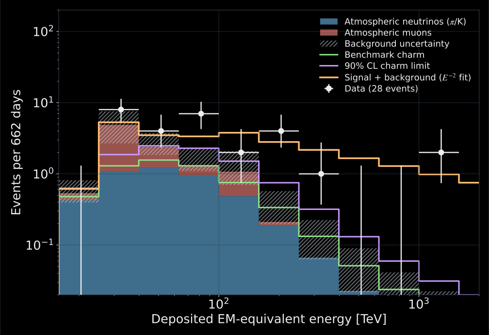
Redrawn IceCube 2013 deposited-energy distribution of 28 starting events, compared with atmospheric muon and neutrino backgrounds and the historical best-fit astrophysical component.

28 events · 662 live days

\[30–1200\,\mathrm{TeV}\]

Deposited energy.

White points: data.

Blue + red: atmospheric backgrounds.

Orange: signal + background.

\[4.1\sigma\]

Benchmark atmospheric hypothesis.

2010–2012 sample and fitted spectrum · Redrawn from the vector artwork of IceCube, Science (2013), Fig. 4
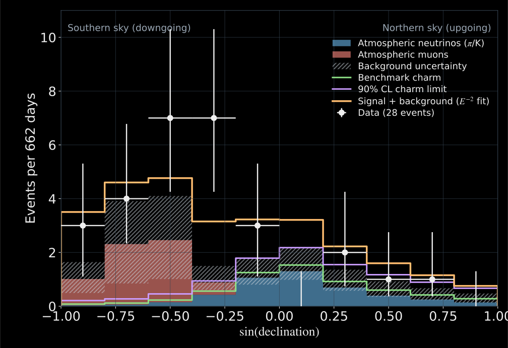
Redrawn IceCube 2013 zenith distribution after the starting-event selection, compared with atmospheric backgrounds and the fitted astrophysical component.

Direction, energy and veto response constrain the background hypothesis together. · Redrawn from the vector artwork

An independent measurement with Baikal-GVD
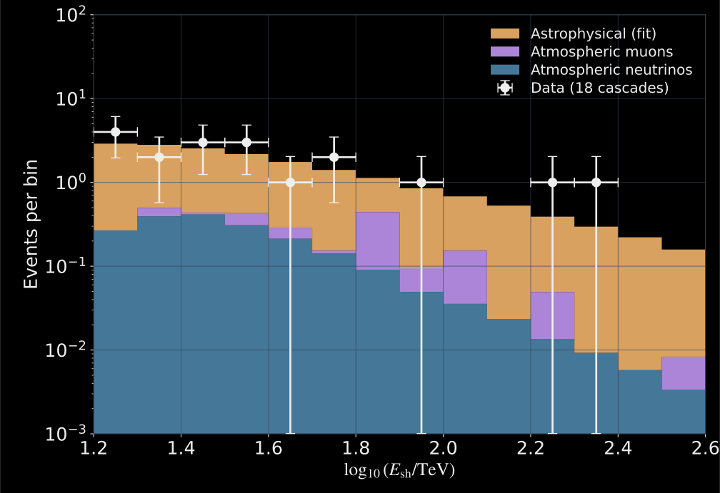
Redrawn Baikal-GVD 2018–2024 upward-going cascade-energy histogram: 18 data events, atmospheric neutrino and muon backgrounds, and the fitted astrophysical contribution.

April 2018–March 2024

18 upward-going cascades

\[E_{\mathrm{sh}}>15\,\mathrm{TeV}\]

Expected atmospheric background:

\[2.8\pm1.0\ \text{events}\]

\[5.1\sigma\]

Points: data · Stacked: fitted signal and backgrounds · Digitized from Baikal-GVD (2025), Fig. 2
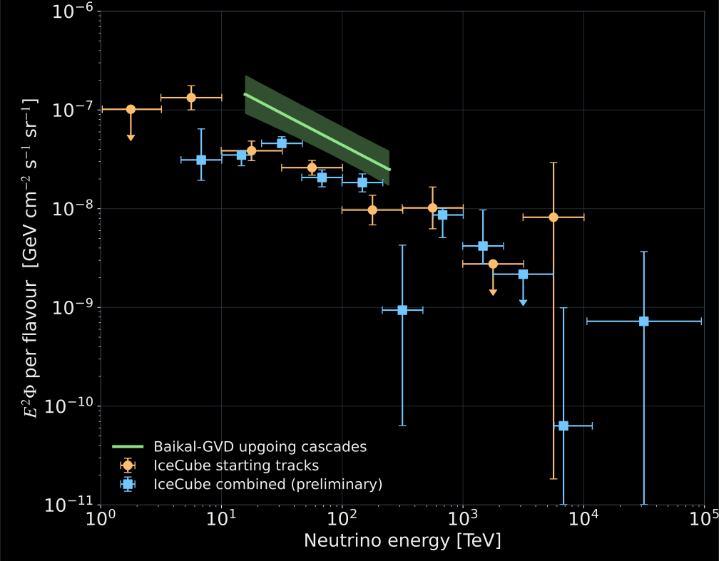
Redrawn GVD spectrum comparison: fitted per-flavour GVD spectrum in green, IceCube starting-track points in orange and preliminary combined-fit points in blue.

Per flavour, \(\nu+\bar\nu\) · Published 2025 comparison · Blue IceCube points are preliminary · Digitized from Fig. 4

The Milky Way in neutrinos
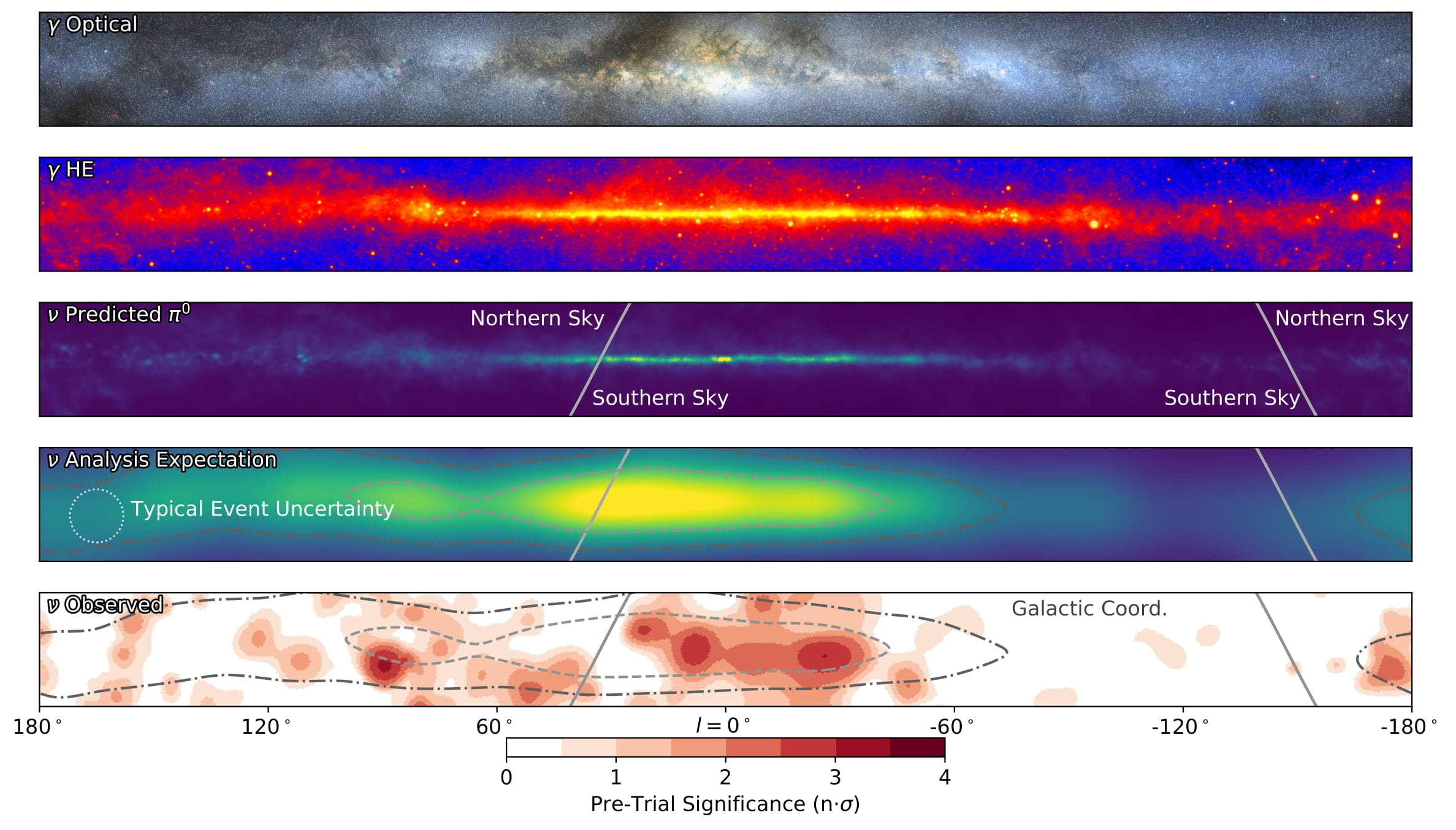
IceCube's five Galactic-coordinate views: optical, gamma rays, predicted neutrino emission, analysis expectation and observed pre-trial significance.

IceCube Collaboration, Science (2023) · Diffuse Galactic emission: \(4.5\sigma\)

ANTARES, 2023: a mild hint of TeV neutrinos from the inner Galactic ridge.
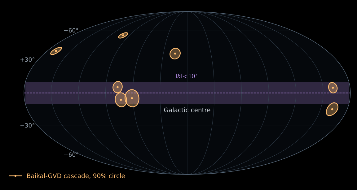
Redrawn sky map in Galactic coordinates: the eight Baikal-GVD cascades above 200 TeV as orange 90% containment circles; five of them lie in or next to the shaded band within 10 degrees of the Galactic plane.

8 cascades above 200 TeV

They crowd towards the Galactic plane.
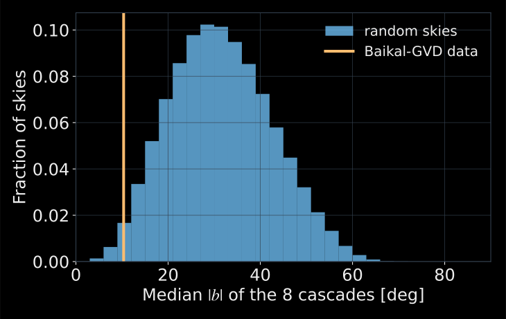
Median absolute Galactic latitude of the eight cascades compared with skies whose right ascensions are randomized: the data line lies in the low tail of the random-sky histogram.

Baikal-GVD: \(p=1.4\times10^{-2}\)

With IceCube: \(p=3.4\times10^{-4}\)

V. A. Allakhverdyan et al. (Baikal-GVD) with Y. Y. Kovalev, A. V. Plavin, D. V. Semikoz, S. V. Troitsky · ApJ 982, 73 (2025) · Redrawn from Table 1; test of Fig. 1 recomputed

Model Galaxy (illustrative) · Baikal-GVD cascades above 200 TeV and the published shuffling test

NGC 1068 and X-ray-bright AGN
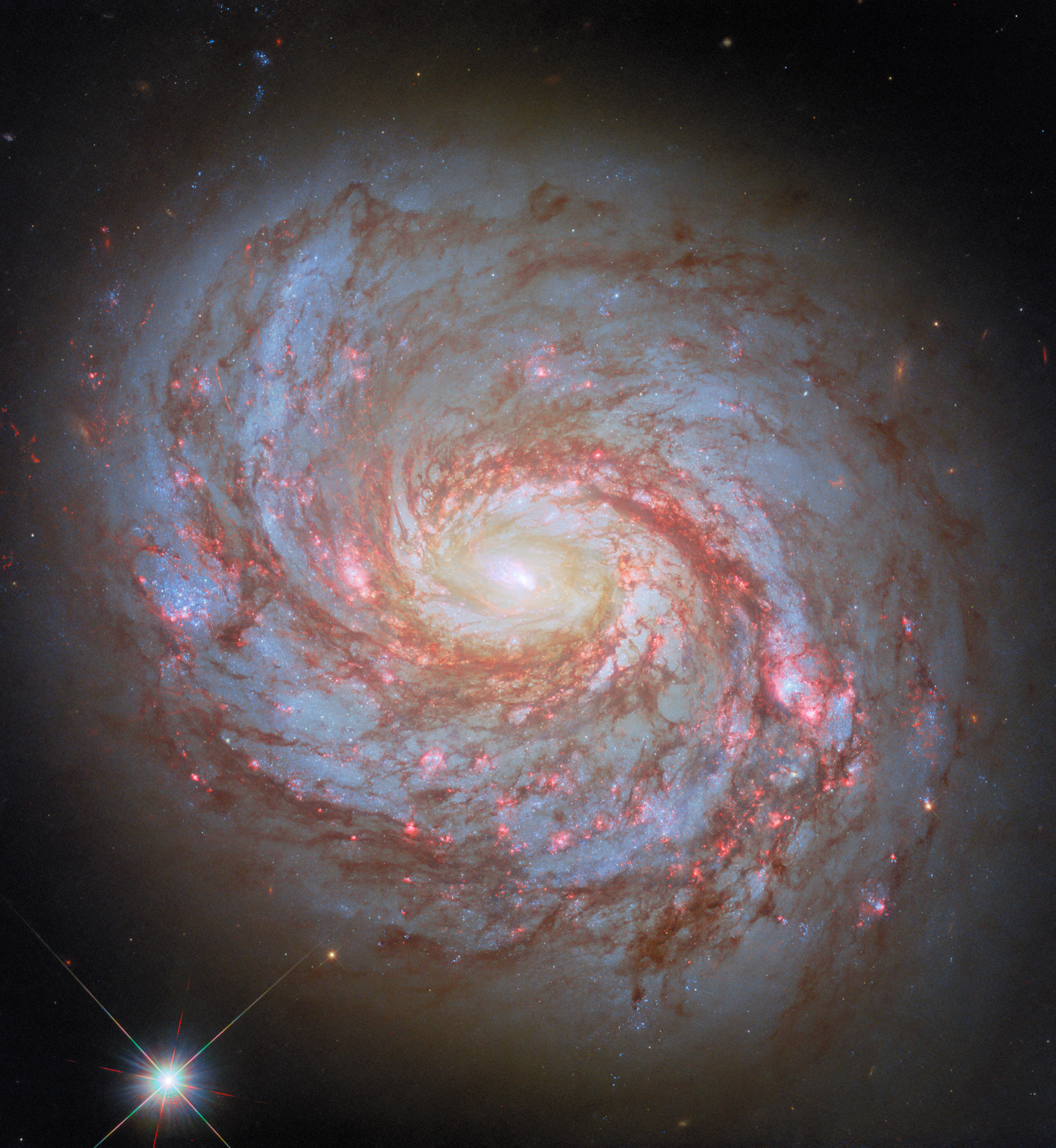
Actual Hubble ultraviolet and optical observations of the spiral galaxy Messier 77, NGC 1068, showing its bright nucleus and dusty spiral arms.

ESA/Hubble & NASA, L. C. Ho, D. Thilker
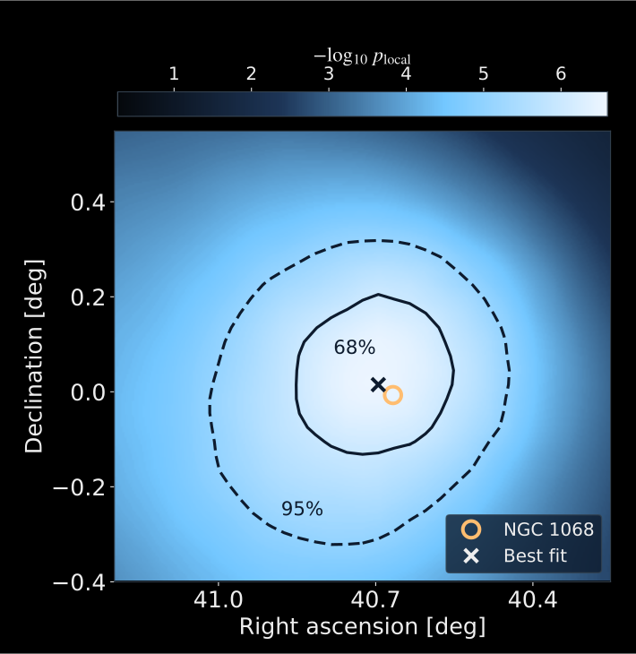
Redrawn latest IceCube fine scan around NGC 1068: local significance map, 68% and 95% contours and the galaxy position. The significance of a preselected catalogue source differs from the significance of an all-sky search.

13.1 years

\[4.0\sigma\]

After catalogue trials.

Seyfert 2

A dust-obscured active nucleus.

Hubble (2025) · IceCube Collaboration · Redrawn from 2026 analysis, Fig. 2
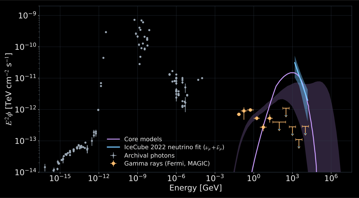
Redrawn NGC 1068 spectral energy distribution from the 2022 IceCube paper: archival photon measurements, Fermi and MAGIC points or limits, the 2022 muon-neutrino fit and two theoretical core models.

Blue: 2022 neutrino fit.

Orange: gamma-ray data and limits.

Violet: core models.

The photon spectrum constrains where pion production can occur.

Historical comparison · \(\nu_\mu+\bar\nu_\mu\), \(95\%\) fit band · Redrawn from IceCube, Science (2022), Fig. 4
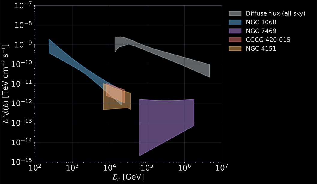
Redrawn IceCube all-flavour spectra of the strongest X-ray-bright AGN, including NGC 1068, compared with the all-sky diffuse neutrino flux. Source spectra and the diffuse spectrum retain the publication's normalization conventions.

All flavours · NGC 1068: \(\Phi_\nu(E)\propto E^{-\gamma}\), \(\gamma=3.4\pm0.2\) · IceCube Collaboration · Redrawn from the vector artwork

Blazars: TXS 0506+056 and radio-bright jets

22 September 2017

IceCube-170922A

Most probable energy

\[E_\nu\sim290\,\mathrm{TeV}\]

Fermi-LAT + MAGIC

A flaring blazar in the neutrino direction.

\(\sim3\sigma\) association

KM3-230213A: an ultra-high-energy event

13 February 2023

ARCA · 21 detection units

Parent neutrino

\[E_\nu\sim220\,\mathrm{PeV}\]

  • Nearly horizontal.
  • No identified counterpart.

KM3NeT Collaboration · Nature (2025)
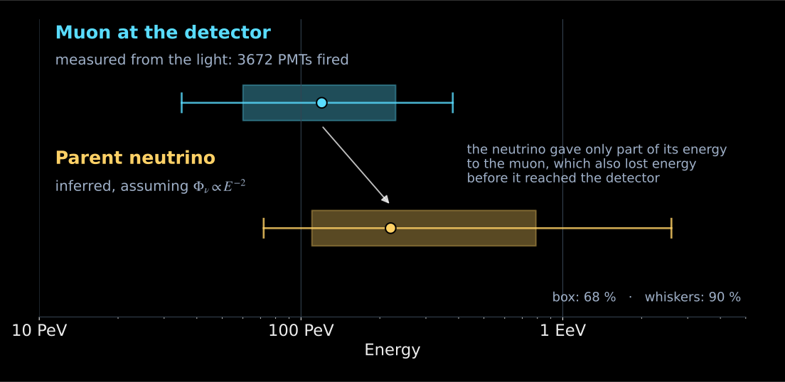
Energy intervals of KM3-230213A drawn from the published numbers: the muon energy at the detector, 120 PeV with a 68 percent interval of 60 to 230 PeV, and the inferred parent-neutrino energy, median 220 PeV with a 68 percent interval of 110 to 790 PeV, assuming an E to the minus 2 spectrum. Whiskers show 90 percent intervals.

Muon at the detector

\[E_\mu=120^{+110}_{-60}\,\mathrm{PeV}\]

\(68\%\) confidence interval

Parent neutrino

Median: \(220\,\mathrm{PeV}\)

Central \(68\%\): \(110–790\,\mathrm{PeV}\)

Assuming \(\Phi_\nu(E)\propto E^{-2}\).

Drawn from the numbers in the text of KM3NeT, Nature (2025) · Their Fig. 2 (CC BY-NC-ND) is kept unmodified for questions

Observatories

Neutrino observatories

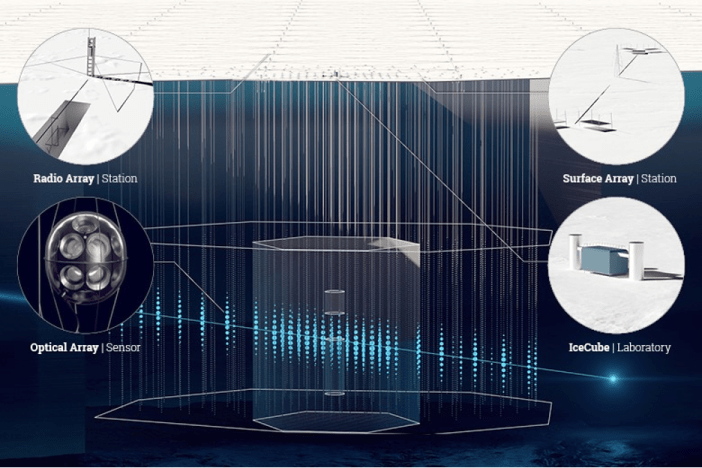
South Pole, Antarctic ice

IceCube: \(1\,\mathrm{km}^3\), operating.

Upgrade: 5 new strings, installed in 2026.

Gen2: \(8\,\mathrm{km}^3\) optical array, proposed.

Measurement: more high-energy events; improved calibration and a radio extension.
Mediterranean Sea

ARCA: \(\sim1\,\mathrm{km}^3\) for neutrino astronomy.

ORCA: \(\sim7\,\mathrm{Mt}\) for neutrino oscillations.

Full design: 230 / 115 strings.

Construction and data taking.

Measurement: source searches with ARCA; oscillations with ORCA.
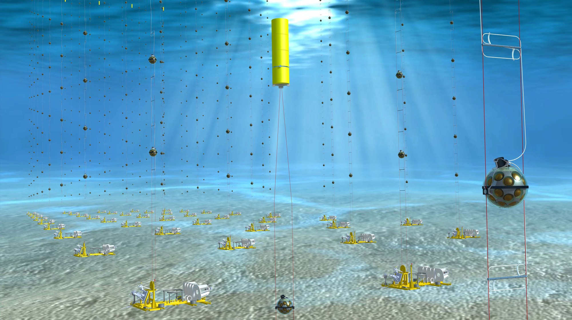
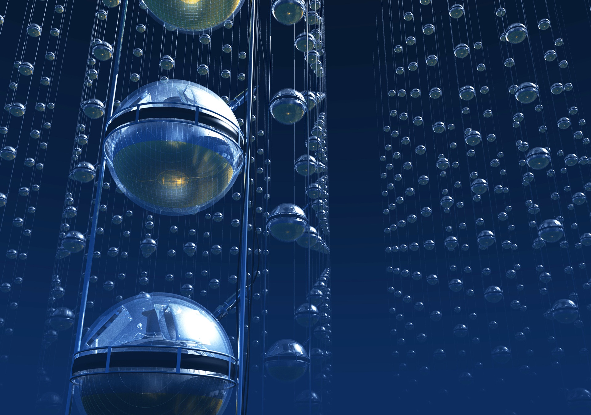
Artist's impression from inside a KM3NeT building block on the sea floor: vertical detection units carrying spherical multi-PMT optical modules, the yellow buoy of a nearby unit, a close-up optical module and anchors on the seabed. An illustration, not a photograph.

Artist’s impression · Edward Berbee/Nikhef · KM3NeT

Lake Baikal, fresh water

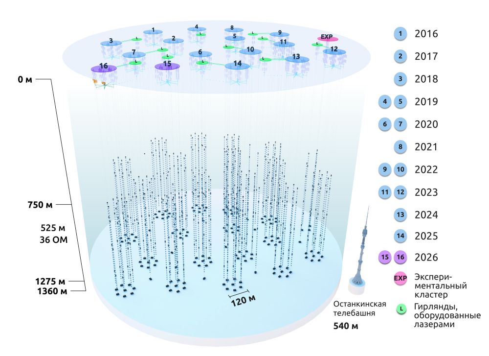
2026: 16 clusters, operating.

Reported effective volume: \(0.8\,\mathrm{km}^3\).

Modular growth through winter deployment.

Measurement: independent diffuse spectra and northern-site source searches.
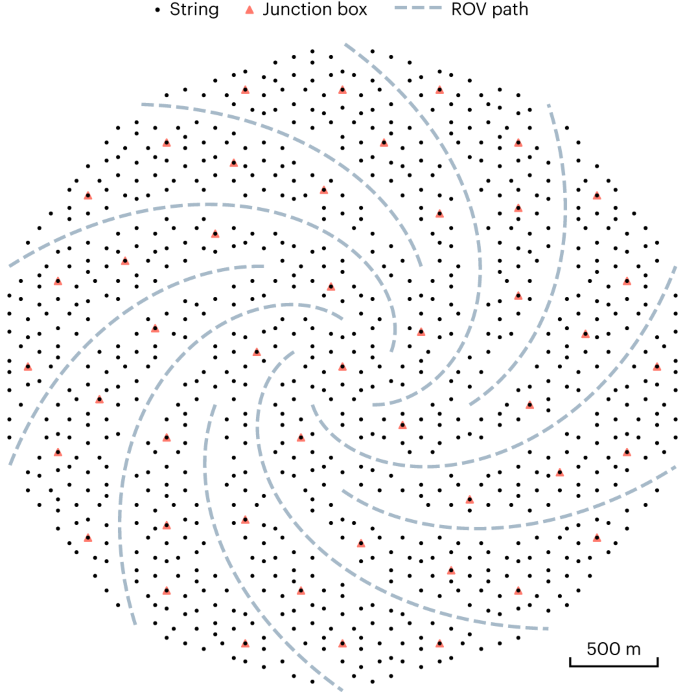
South China Sea

Design: \(7.5\,\mathrm{km}^3\), 1,211 strings.

Sensors: hybrid PMT + SiPM modules.

R&D and pathfinder programme.

Design goal: photon timing and directional information from hybrid sensors.
China + Russia

Design: \(\sim30\,\mathrm{km}^3\).

Sensors: 20-inch PMTs.

The Baikal option, B-HUNT, is the next slide.
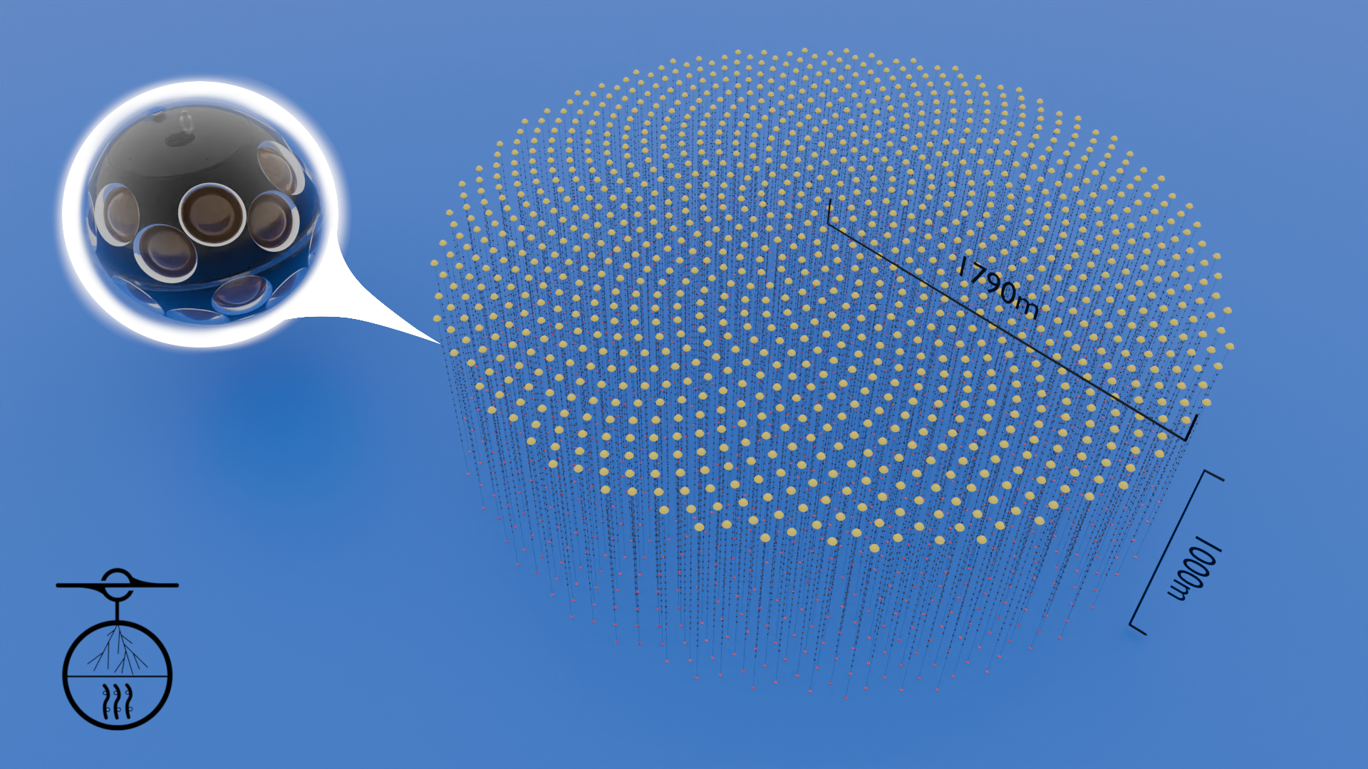
South China Sea

Design: \(10\,\mathrm{km}^3\), 1,200 strings.

Sensors: multi-PMT optical modules.

Proposal and hardware R&D.

Design goal: high-energy source searches with a large multi-PMT array.
Baikal-GVD → B-HUNT
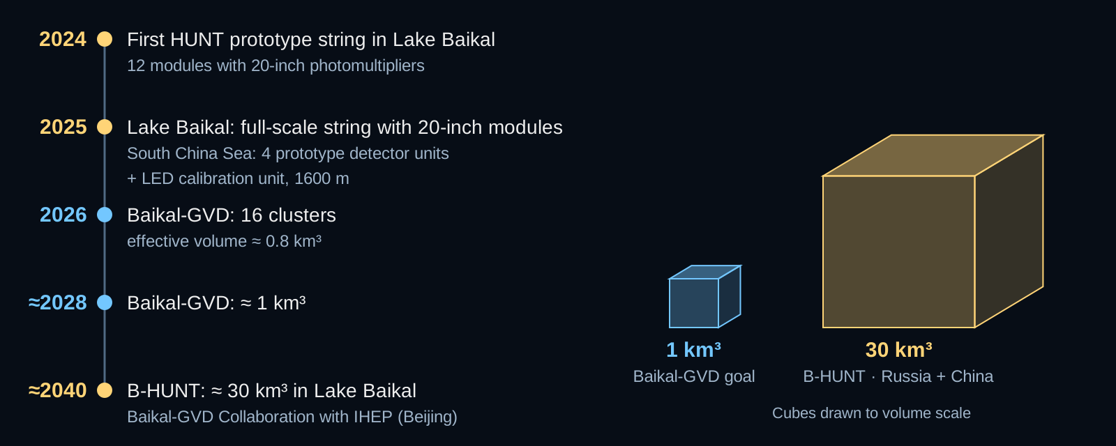
Milestones: 2024 first HUNT prototype string in Lake Baikal with 12 modules of 20-inch photomultipliers; 2025 a full-scale string with 20-inch modules operating in Lake Baikal, and four prototype detector units with an LED calibration unit at 1600 metres in the South China Sea; 2026 Baikal-GVD with 16 clusters and about 0.8 cubic kilometres effective volume; about 2028 Baikal-GVD at about 1 cubic kilometre; about 2040 B-HUNT at about 30 cubic kilometres. Two cubes of 1 and 30 cubic kilometres are drawn to volume scale.

Russia + China · Baikal-GVD Collaboration with IHEP (Beijing) · JINR (2026) · IHEP

The ice is a platform: strings are deployed from the frozen lake every winter.

Water: light scatters less than in ice, so cascade directions are sharper.

Northern site: the Galactic Centre is below the horizon \(75\%\) of the day.

A gamma-ray partner: LHAASO watches the same northern sky.

Alerts and follow-up: work in progress.

Prospects

What we want to discover

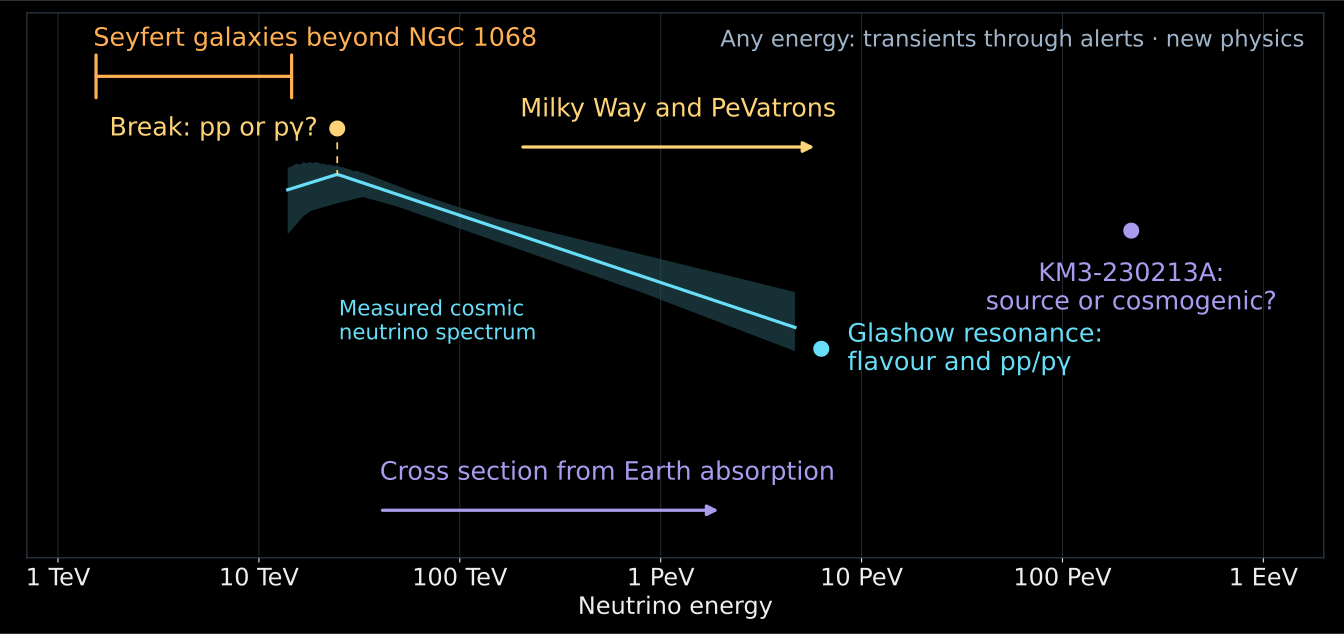
Open questions placed on a neutrino-energy axis from 1 TeV to 1 EeV over the measured cosmic neutrino spectrum: Seyfert galaxies beyond NGC 1068 at 1.5 to 15 TeV; the spectral break near 25 TeV, pp or p-gamma; the Milky Way and PeVatrons above 200 TeV; the neutrino cross section from Earth absorption above 40 TeV; the Glashow resonance at 6.3 PeV; and KM3-230213A at about 220 PeV, source or cosmogenic. Transients through alerts and new physics can appear at any energy.

  • Are there more NGC 1068-like Seyferts?
  • What breaks the spectrum near \(25\,\mathrm{TeV}\): \(pp\) or \(p\gamma\)?
  • Which PeVatrons live in the Milky Way?
  • Is KM3-230213A a source or cosmogenic?

Questions on the energy axis · Spectrum: IceCube (2026) · Glashow: IceCube (2021) · KM3-230213A: KM3NeT (2025)

What we lack

  • Northern exposure beyond \(10\,\mathrm{km}^3\): faint sources and the Galactic Centre seen through the Earth
  • Sharper cascade directions: all flavours point back to sources
  • More events above \(1\,\mathrm{PeV}\): the spectrum’s end, Glashow events, the \(100\,\mathrm{PeV}\) puzzle
  • Global alerts, joint analyses, open data: one sky, several telescopes
  • Calibrated optics of water and ice: energies and directions we can trust
  • Population theory within the gamma-ray budget: turning many faint hints into sources
  • People: telescopes are built and understood by people. The programme ФНАФЧ: courses on teach-in.ru

Where are the sources?

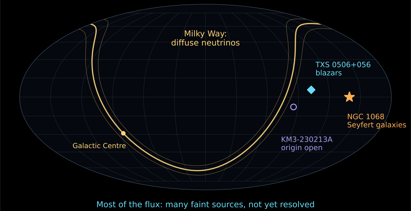
Equatorial sky map. The Galactic plane with the Galactic Centre is marked as diffuse neutrino emission from the Milky Way. NGC 1068 stands for Seyfert galaxies, TXS 0506+056 for blazars, and an open circle marks the direction of KM3-230213A, whose origin is open. Caption: most of the flux comes from many faint sources, not yet resolved.

  • Found: our Galaxy, NGC 1068 and Seyfert galaxies, blazar candidates
  • Still open: most of the flux: a crowd of faint sources
  • Next: bigger telescopes and networks: B-HUNT, KM3NeT, IceCube-Gen2

We have found where to look. Next we must resolve the crowd.

Positions: Baikal-GVD source list (2026) · Evidence: result slides of this lecture

Summary: where we are

  • What do we have?
    • A diffuse astrophysical neutrino flux, seen by IceCube and by Baikal-GVD
    • Neutrinos from our Galaxy, from the Seyfert galaxy NGC 1068 and from blazar candidates
    • One event near \(220\,\mathrm{PeV}\), KM3-230213A
  • Why does it matter?
    • Neutrinos fly straight and leave even dense sources that hide their gamma rays
    • They show where cosmic rays are accelerated

Summary: what next

  • What do we not know?
    • Where most of the flux comes from: a crowd of faint sources
    • What the spectral break near \(25\,\mathrm{TeV}\) means, \(pp\) or \(p\gamma\)
    • Whether KM3-230213A is a source or cosmogenic
  • What must be done?
    • Northern exposure beyond \(10\,\mathrm{km}^3\), sharper cascade directions
    • More events above \(1\,\mathrm{PeV}\), joint analyses and open data
  • When?
    • 2026: Baikal-GVD with \(0.8\,\mathrm{km}^3\), the IceCube Upgrade
    • About 2028: Baikal-GVD at \(1\,\mathrm{km}^3\); about 2040: B-HUNT at \(30\,\mathrm{km}^3\)

Backup

What creates the light?

\(\nu_\mu+N\longrightarrow\mu^-+X.\)

\(\nu_e+N\longrightarrow e^-+X.\)

Cherenkov light

Gold: charge. Blue circles: wavefronts. White: common front. Cyan arrows: light.

Light gets ahead — \(v<c/n\)

The particle gets ahead — \(v>c/n\)
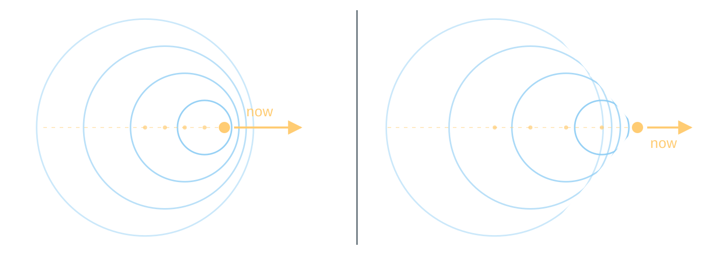
Same-age wavefronts: below threshold the circles are nested; above threshold they share a tangent front behind the particle.

The charge disturbs the medium. A fast charge leaves a common wavefront behind.
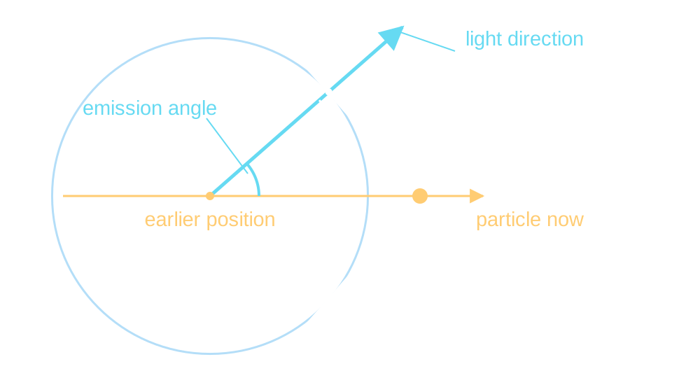
Light travels along a radius of a spherical wavefront, perpendicular to the common tangent front. The emission angle is measured from the forward particle track.

Light goes across the front — not along it.

\[ \cos\theta_C=\frac{c}{nv} \qquad\Longrightarrow\qquad \theta_C\simeq41^\circ\ \text{in water, for }v\simeq c. \]

One photon, a measurable pulse

IceCube
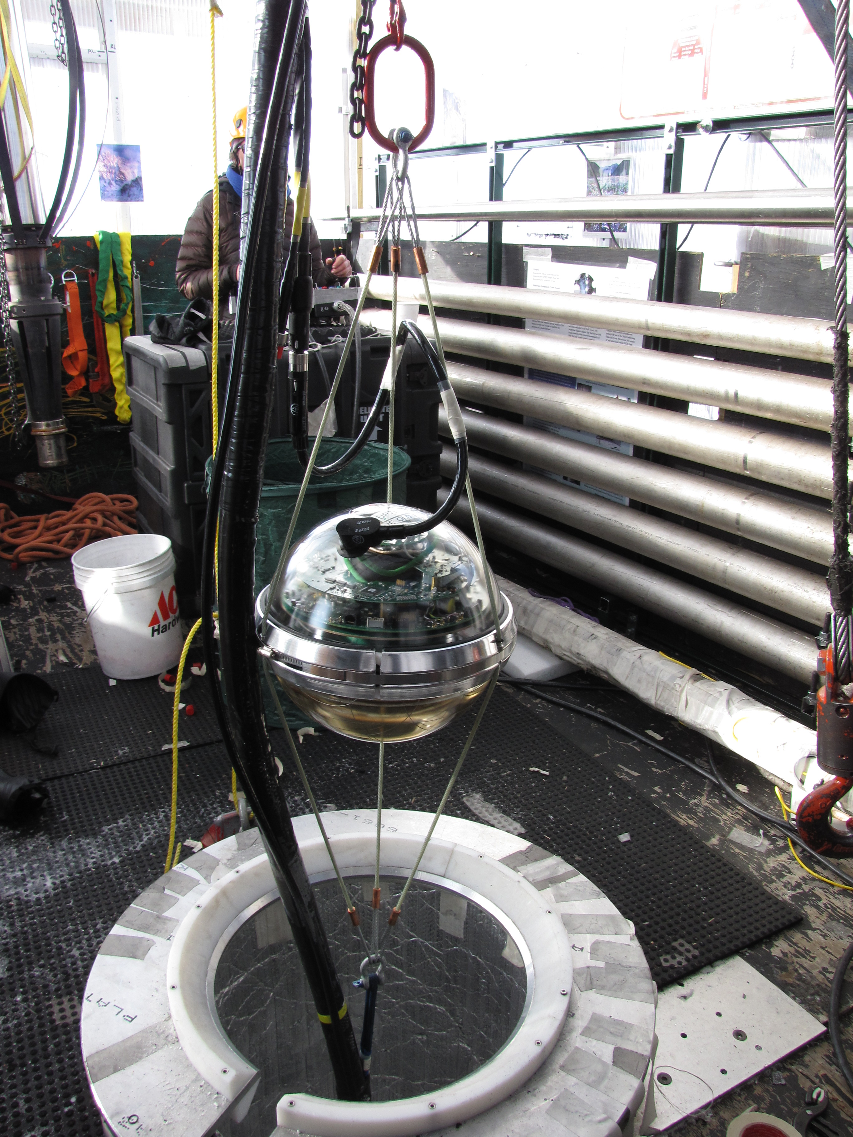
An actual original IceCube DOM during deployment, with one large PMT inside a glass pressure sphere.

One \(10\,\mathrm{inch}\) PMT.

IceCube/NSF.

KM3NeT
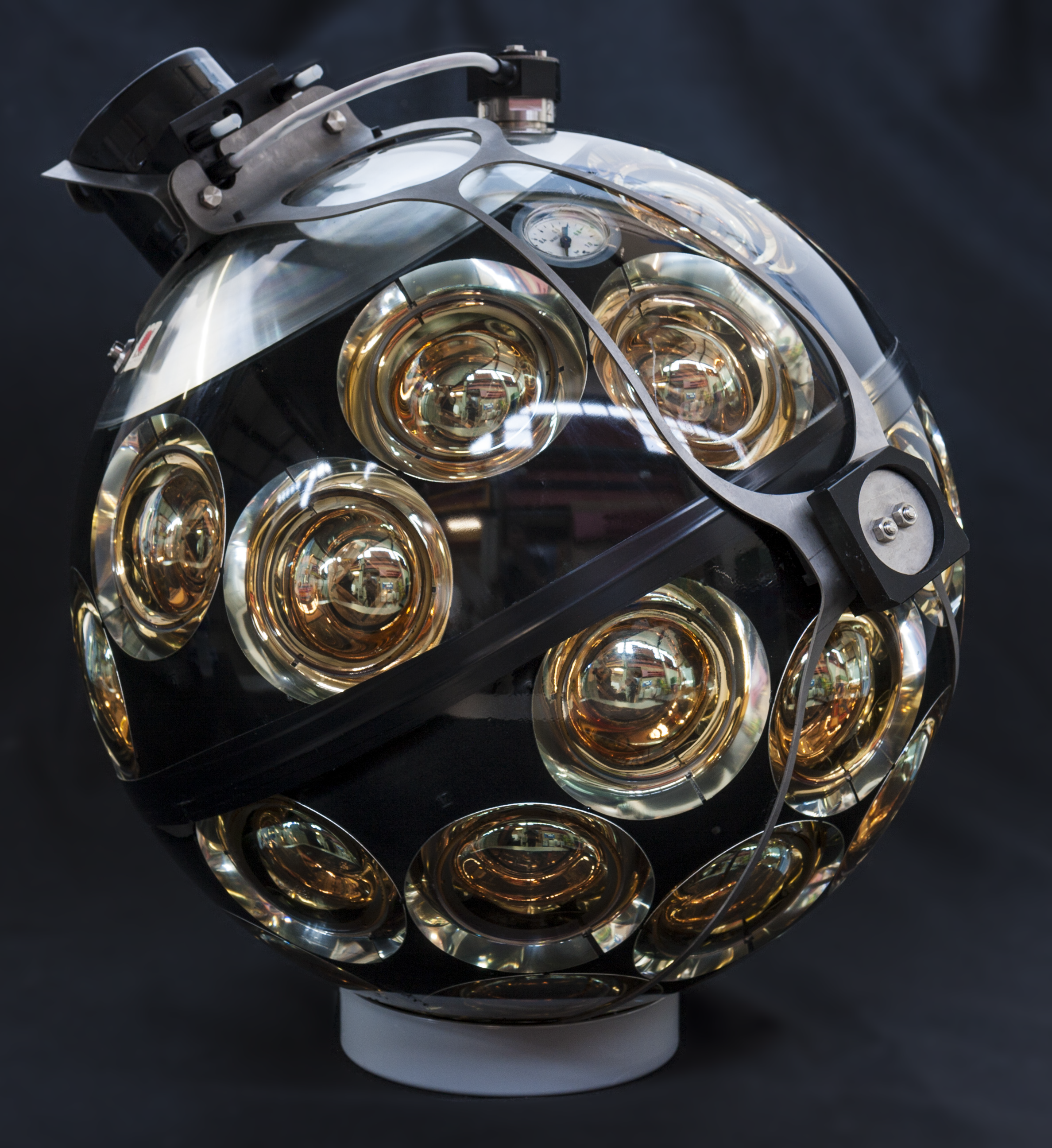
An actual KM3NeT digital optical module with many small PMTs pointing in different directions.

\(31\) three-inch PMTs.

Courtesy KM3NeT.

Baikal-GVD
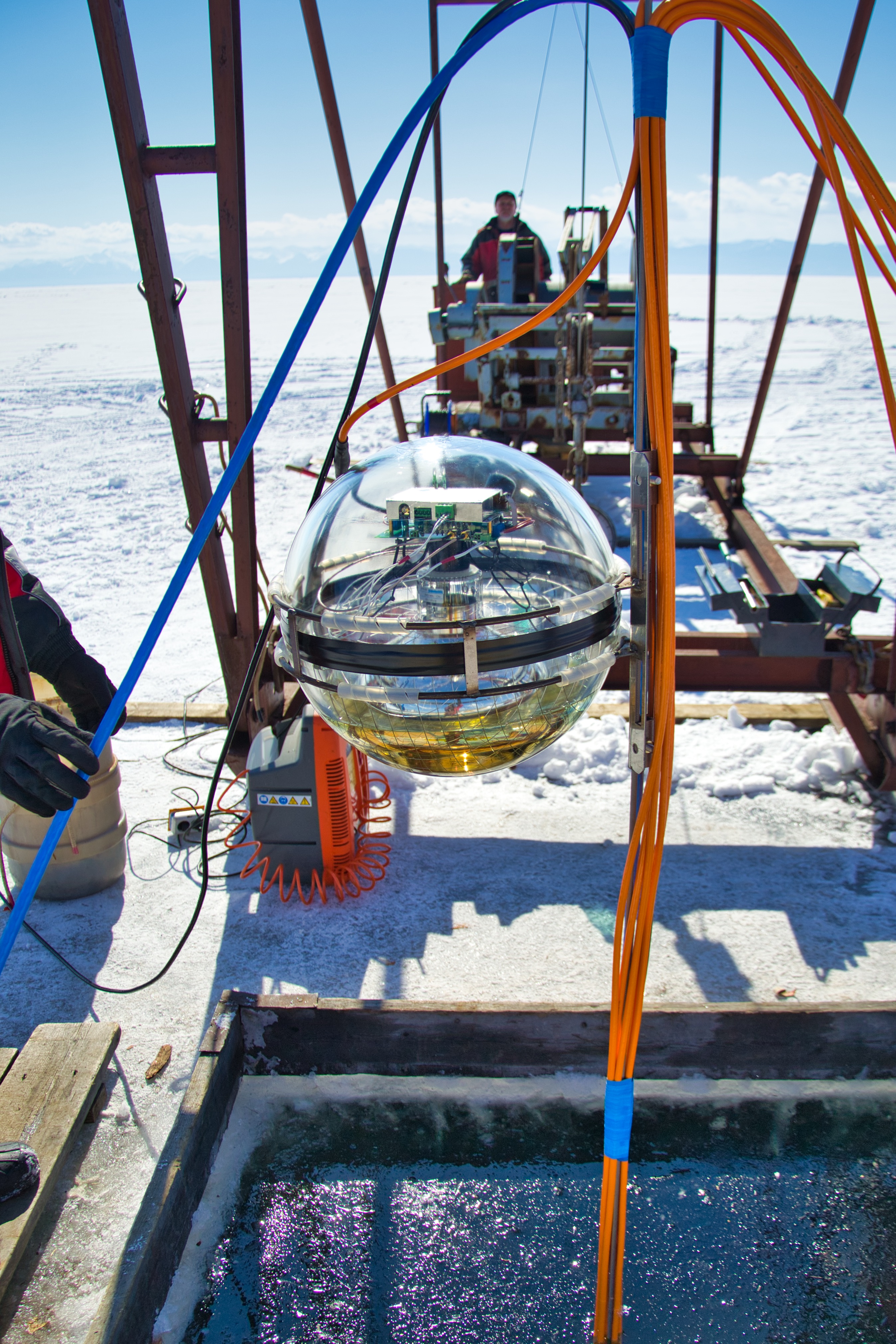
A real Baikal-GVD optical module above an ice hole during deployment, from DN's 2021 lecture.

One \(10\,\mathrm{inch}\) PMT.

Baikal-GVD; supplied by DN.

TRIDENT
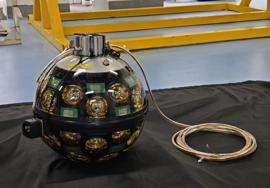
An actual TRIDENT hybrid optical-module prototype in the laboratory, combining PMTs with small SiPM assemblies.

PMTs + SiPMs. Prototype.

TRIDENT / TDLI, SJTU.

Reconstructing an event

Next event:Fit model:

Loading the synthetic event…
Synthetic water detector · crossing point is known · fit direction and time, not vertex or energy

Predict a time for each sensor

\[ \cos\theta_C=\frac{1}{\beta n_{\rm phase}},\qquad t_i^{\rm pred}=t_0+\frac{s_i}{\beta c}+\frac{n_{\rm group}D_i}{c}. \]

\(s_i\): muon distance from the known crossing point to emission.

\(D_i\): photon path from emission to the sensor.

The cone uses the phase index; flight time uses the group index.

Find the direction that agrees with the signals

\[ S=\frac{1}{2\sigma_t^2}\sum_{i,k} \left(t_{ik}^{\rm obs}-t_i^{\rm pred}\right)^2 \longrightarrow\min_{\theta,\phi,t_0}. \]

Every detected photoelectron contributes a measured time.

Here: known crossing point, straight muon, homogeneous medium. Only direction and time offset are fitted — not vertex or energy.

How does a wrong model of the medium change the inferred direction?

Synthetic teaching model, not an experiment’s reconstruction or an angular-resolution forecast. The arrow is the muon’s direction of travel; the source direction is opposite.

Backgrounds

Telescope Optical background Pulses / PMT Muon-dominated samples
IceCube PMT + glass noise \(0.56\,\mathrm{kHz}\) · 10-inch \(2.7\,\mathrm{kHz}\) · IC86 DAQ
KM3NeT \(^{40}\mathrm K\) + bioluminescence \(\sim7\,\mathrm{kHz}\) · 3-inch \(\sim1\,\mathrm{Hz}\) · ARCA6 reconstructed
Baikal-GVD Water luminescence \(20–100\,\mathrm{kHz}\) · 10-inch \(\sim3\,\mathrm{Hz/cluster}\) · reconstructed

Pulses, DAQ triggers and reconstructed events are different counting levels. IceCube · KM3NeT · Baikal-GVD
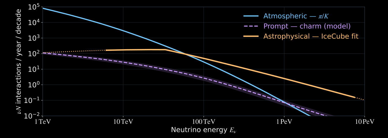
Calculated neutrino-nucleon interactions per year per energy decade in one cubic kilometre of water from the downward hemisphere, before event selection. Conventional atmospheric neutrinos fall more steeply than the astrophysical component. A dashed prompt-charm prediction has a shaded theoretical band. Astrophysical best-fit extrapolations outside the sensitive range are dotted.

\(1\,\mathrm{km^3}\) water · downward \(2\pi\) · all flavours, \(\nu+\bar\nu\) · CC+NC · before selection.

From events to a neutrino flux
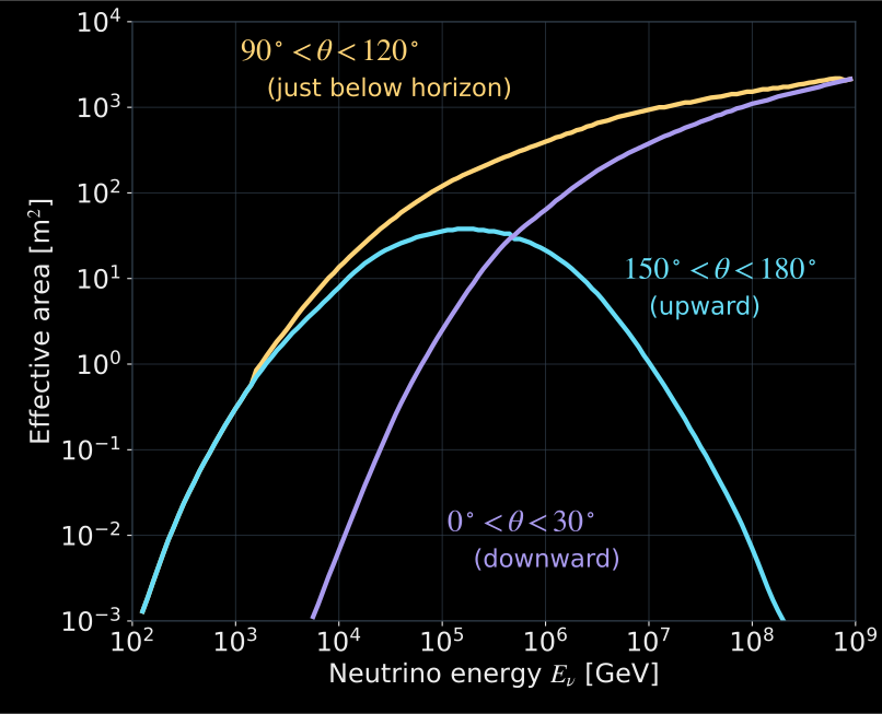
Illustrative IceCube point-source effective-area curves versus true neutrino energy for three zenith intervals, redrawn from curves digitized from the published review figure. Selection suppresses low-energy downgoing events; Earth absorption suppresses the highest-energy vertically upgoing events.

Near the horizon: short Earth chord.

Upward: Earth absorption at high energy.

Downward: atmospheric-muon rejection.

\(A_{\mathrm{eff}}\) includes interaction, propagation and event selection.

\[ N=T\sum_\alpha\int dE_\nu\,d\Omega\, \Phi_\alpha(E_\nu,\Omega)\,A_{\mathrm{eff},\alpha}(E_\nu,\Omega) \]

Illustrative point-source selection · Redrawn, digitized from Spiering (2026), Fig. 6
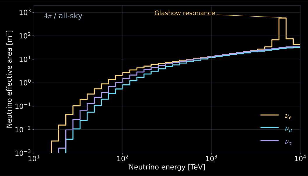
IceCube 2013 all-sky-averaged effective areas by flavour for contained starting events, in square metres versus neutrino energy in TeV, redrawn from the step histogram digitized from the published figure. The electron-flavour peak at 6.3 PeV is the Glashow resonance.

A specific sample

  • Start inside the fiducial volume.
  • Reject early light at the boundary.
  • The accepted events determine the response used in the flux fit.

Historical HESE selection, 2010–2012 · Redrawn, digitized from IceCube (2013), Fig. 7

Event Light constrains Parent-neutrino inference
Contained \(\nu_e\) CC Electromagnetic + hadronic deposits \(E_{\mathrm{dep}}\simeq E_\nu\), after response calibration
Through-going \(\mu\) Muon energy losses inside the array \(E_\mu\) at the detector, then a spectrum-dependent \(E_\nu\) distribution
Neutral current Hadronic deposit \(E_{\mathrm{dep}}\sim yE_\nu\); outgoing neutrino is unseen

Historical HESE reconstruction (2013): tracks \(<1^\circ\); cascades \(10–15^\circ\).

Quoted median angular scales above about \(50\,\mathrm{TeV}\). Neutrino–muon kinematics adds a separate spread.

\(y\): inelasticity · IceCube reconstruction (2013)

Point-source searches: Baikal-GVD

988 tracks · 92 directions · April 2019–March 2024
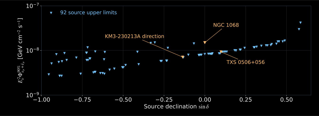
The 92 Baikal-GVD E^-2 source flux limits from published Table 1, drawn versus sine of declination at 90% confidence. NGC 1068, TXS 0506+056 and the KM3-230213A direction are highlighted. This graph contains only observed source limits, not a new sensitivity calculation.

\(E^{-2}\) spectrum · \(90\%\) CL · No significant catalogue excess · Baikal-GVD (2026), Table 1

Real-time alerts and multimessenger follow-up with Baikal-GVD: work in progress.
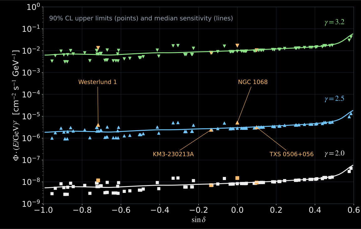
Redrawn Baikal-GVD figure 2: 90% source limits and median expected sensitivities for spectral indices 2, 2.5 and 3.2. Symbols are limits; solid curves are sensitivities.

Symbols: source limits · Lines: expected sensitivity · Baikal-GVD (2026), Fig. 2 · Limits from Table 1, sensitivities redrawn from the vector artwork
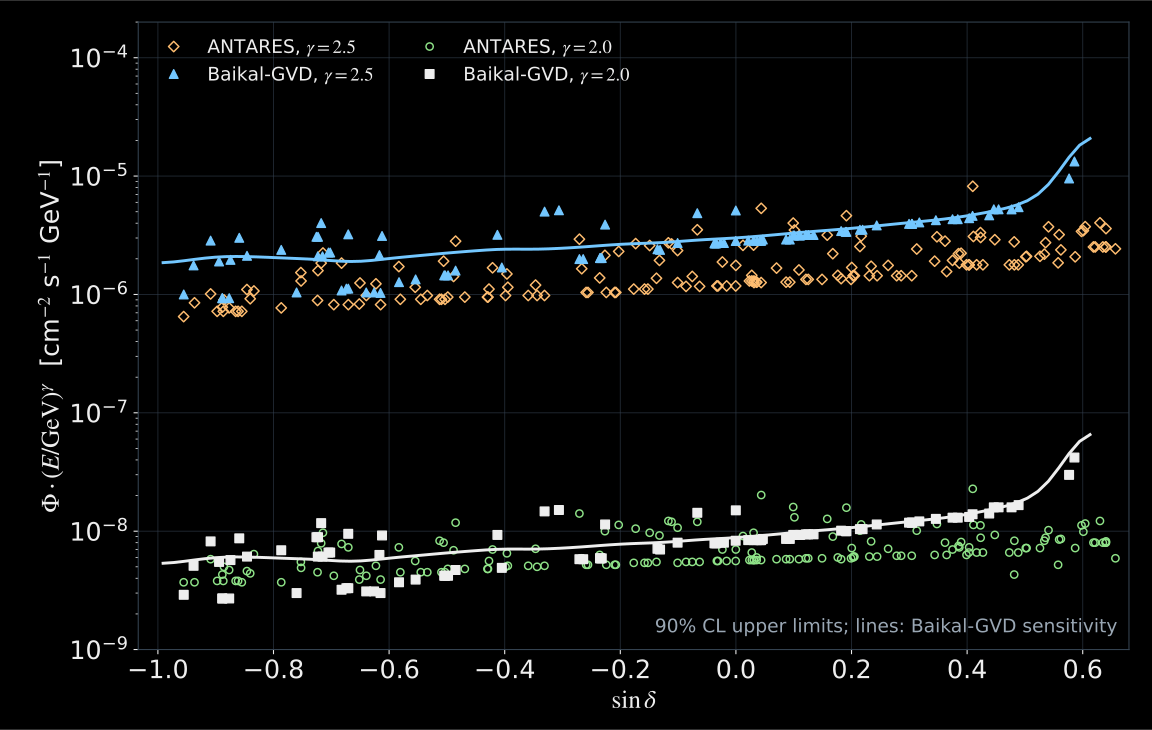
Redrawn comparison of Baikal-GVD and ANTARES 90% point-source limits for E^-2 and E^-2.5 spectra, with the declination axis of the original. This compares selected analysis samples, not equal-volume instruments.

Matched spectral assumptions · Baikal-GVD Collaboration (2026), Fig. 3 · Redrawn from the vector artwork; Baikal-GVD limits from Table 1

A global view of the neutrino sky
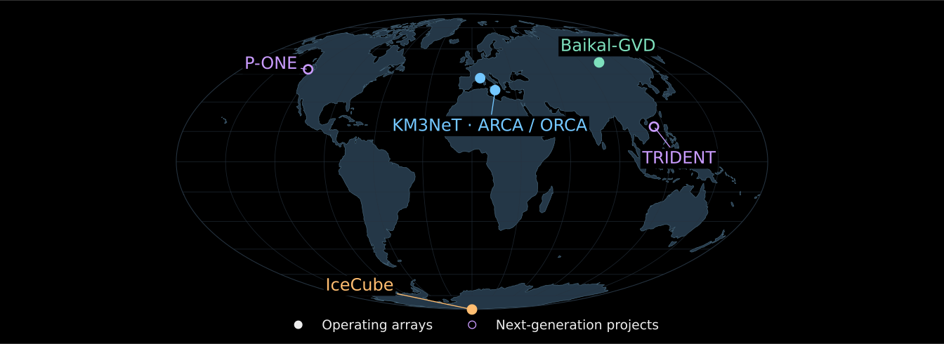
Mollweide world map of operating IceCube, KM3NeT ARCA and ORCA, and Baikal-GVD sites, with open markers for P-ONE's Cascadia region and the TRIDENT design site. Open markers denote next-generation projects, not completed operating arrays.

Site overview · October 2026 · coastlines: Natural Earth
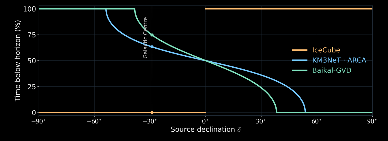
Calculated fraction of a sidereal day each source spends below the horizon of IceCube, ARCA and Baikal-GVD versus declination. At the Galactic Centre the fractions are 0%, 63% and 75%, respectively. This is geometry, not effective area or sensitivity.

Geometry only, not sensitivity · IceCube also observes the southern sky with starting and contained events.
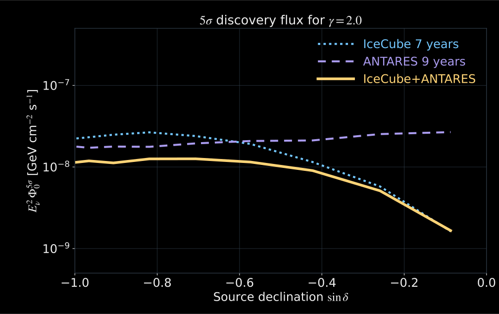
ANTARES–IceCube joint-search E^-2 discovery-flux comparison, redrawn from digitized published curves: the combined gold curve is lower than the separate seven-year IceCube and nine-year ANTARES curves in the southern sky. The ordinate is the five-sigma discovery flux, not a detected source flux.

IceCube · 7 years

ANTARES · 9 years

  • Gold: joint analysis.
  • Lower flux = better discovery potential.
  • Assumed spectrum: \(E^{-2}\).

Published joint analysis, not a next-generation projection · Redrawn, digitized from ANTARES & IceCube (2020), Fig. 2