Notebook: VEGAS и обычный Монте-Карло

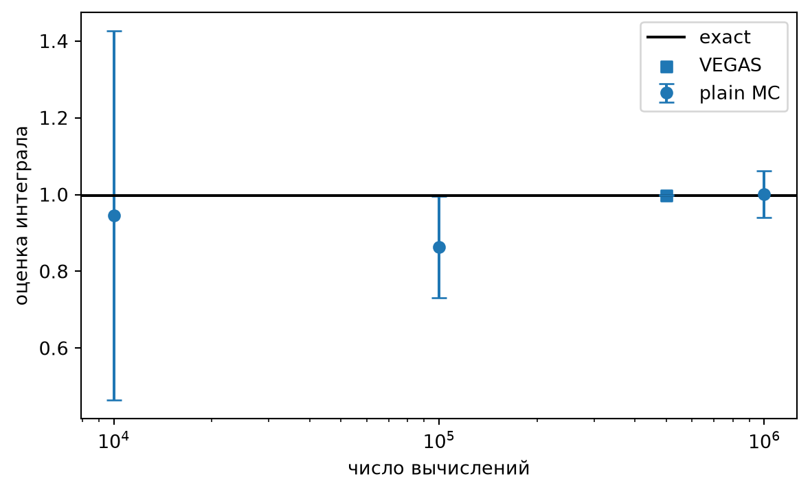
Этот notebook воспроизводит пример из лекции 07: интеграл от узкого многомерного пика в единичном гиперкубе. Сравниваем обычный Монте-Карло, тензорную квадратуру Gauss–Legendre и адаптивный интегратор VEGAS.

1 Общий код примера

Один и тот же код используется в слайдах и в этом notebook.

from pathlib import Path
import runpy

def find_demo_script():
    candidates = [
        Path("../../shared/notebooks/mc_vegas_demo.py"),
        Path("../../../shared/notebooks/mc_vegas_demo.py"),
        Path("shared/notebooks/mc_vegas_demo.py"),
    ]
    for path in candidates:
        if path.exists():
            return path
    raise FileNotFoundError("mc_vegas_demo.py was not found")

demo_path = find_demo_script()
demo = runpy.run_path(str(demo_path))

exact_integral = demo["exact_integral"]
plain_mc = demo["plain_mc"]
tensor_gauss = demo["tensor_gauss"]
vegas_result = demo["vegas_result"]

exact = exact_integral()
print(f"demo script: {demo_path}")
print(f"d = {demo['d']}, sigma = {demo['sigma']}")
print(f"exact = {exact:.12g}")

demo script: ../../../shared/notebooks/mc_vegas_demo.py
d = 8, sigma = 0.1
exact = 0.997819635914

2 Обычный Монте-Карло

Равномерная генерация не знает, где находится пик. Она остаётся несмещённой в ансамбле, но дисперсия может быть большой.

import pandas as pd

plain_rows = []
for N in [10_000, 100_000, 1_000_000]:
    value, error = plain_mc(N)
    plain_rows.append({
        "N": N,
        "estimate": value,
        "stat_error": error,
        "pull": (value - exact) / error,
    })

plain_table = pd.DataFrame(plain_rows)
plain_table

	N	estimate	stat_error	pull
0	10000	0.945546	0.480515	-0.108787
1	100000	0.863792	0.131991	-1.015425
2	1000000	1.000935	0.060680	0.051339

3 Tensor-product Gauss–Legendre

В большой размерности проблема регулярной квадратуры не в формуле, а в числе узлов: при (m) узлах на координату требуется (m^d) вычислений.

grid_rows = []
for m in [3, 5, 7]:
    value, calls = tensor_gauss(m)
    grid_rows.append({
        "nodes_per_axis": m,
        "calls": calls,
        "estimate": value,
        "relative_bias": (value - exact) / exact,
    })

grid_table = pd.DataFrame(grid_rows)
grid_table

	nodes_per_axis	calls	estimate	relative_bias
0	3	6561	0.589148	-0.409564
1	5	390625	0.722156	-0.276266
2	7	5764801	0.963411	-0.034483

4 VEGAS

VEGAS сначала адаптирует разбиение координат, а затем оценивает интеграл уже после адаптации. Он не меняет закон (1/N), но может сильно уменьшить коэффициент перед статистической ошибкой.

result = vegas_result()
print(f"VEGAS = {result}")
print(f"Q     = {result.Q:.3f}")

VEGAS = 0.99787(53)
Q     = 0.428

5 Сравнение

comparison = pd.DataFrame([
    {
        "method": "plain MC, N=1e6",
        "estimate": plain_table.loc[plain_table["N"] == 1_000_000, "estimate"].iloc[0],
        "error_or_bias": plain_table.loc[plain_table["N"] == 1_000_000, "stat_error"].iloc[0],
    },
    {
        "method": "Gauss-Legendre, m=7",
        "estimate": grid_table.loc[grid_table["nodes_per_axis"] == 7, "estimate"].iloc[0],
        "error_or_bias": grid_table.loc[grid_table["nodes_per_axis"] == 7, "relative_bias"].iloc[0],
    },
    {
        "method": "VEGAS",
        "estimate": result.mean,
        "error_or_bias": result.sdev,
    },
])

comparison

	method	estimate	error_or_bias
0	plain MC, N=1e6	1.000935	0.060680
1	Gauss-Legendre, m=7	0.963411	-0.034483
2	VEGAS	0.997873	0.000529

import matplotlib.pyplot as plt

fig, ax = plt.subplots(figsize=(7.0, 4.0))
ax.errorbar(
    plain_table["N"],
    plain_table["estimate"],
    yerr=plain_table["stat_error"],
    fmt="o",
    capsize=4,
    label="plain MC",
)
ax.axhline(exact, color="black", linewidth=1.5, label="exact")
ax.scatter([500_000], [result.mean], marker="s", label="VEGAS")
ax.errorbar([500_000], [result.mean], yerr=[result.sdev], fmt="none", capsize=4)
ax.set_xscale("log")
ax.set_xlabel("число вычислений")
ax.set_ylabel("оценка интеграла")
ax.legend()
plt.show()