Lecture 1. Motivation and course overview

Statistical Data Analysis

Dmitry V. Naumov (JINR)

Lecture Plan

• Can you read these typical plots in modern physics?

Disclaimer

• I am not a statistician. I am a physicist who uses statistical analysis in practice.
• I will introduce the main concepts, tricks, and the language physicists use when talking to each other:
  • I discovered a signal with 5 \(\sigma\) significance!
  • We observe an excess in the data.
  • No significant excess is seen.
  • We exclude this region of parameter space at 95% C.L.
  • We set an upper limit on the cross section.
  • The fit converged nicely.
  • The dominant uncertainty is systematic.
  • Correlations between bins are important.
  • These nuisance parameters were profiled in the fit.
  • We must use the full covariance matrix.

Notations

• Scalars will be denoted by italic letters: \(x\), \(y\), \(\theta\)

• Vectors will be denoted in boldface: \(\mathbf{x}=(x_1,x_2,\dots,x_n)\)

• Matrices will be denoted in boldface capitals: \(\mathbf{V}\), \(\mathbf{M}\)

• Random variables will be denoted by capital letters: \(X\), \(Y\)

• Their observed values will be denoted by lowercase letters: \(x\), \(y\)

• Probability of an event \(A\) will be denoted by \(P(A)\)

• Probability density function will be denoted by \(f(x)\) or \(p(x)\)

• Model parameters will be denoted by \(\theta\)

• Estimated values of parameters will be denoted by \(\widehat{\theta}\)

Notations (continued)

• Expectation value: \(\mathbb{E}[X]\)

• Variance: \(\mathrm{Var}(X)\)

• Standard deviation: \(\sigma_X=\sqrt{\mathrm{Var}(X)}\)

• Covariance: \(\mathrm{cov}(X,Y)\)

• Correlation coefficient: \(\rho(X,Y)\)

Frequentist vs Bayes

There are two schools that treat probability differently.

• Relative frequency (Frequentist)
  \(A\), \(B\), … are outcomes of a repeatable experiment.

  \[ P(A)=\lim\limits_{n\to\infty}\frac{\text{number of times outcome is }A}{n} \]

• Subjective probability (Bayes)

  \[ P(A)=\text{degree of belief that }A\text{ is true} \]

  \[ P(A\mid B)=\frac{P(B\mid A)\,P(A)}{P(B)} \]

• In this course I will talk mainly about Frequentist statistics.

Literature

• Particle Data Group: Review of statistics (2015)

• G. Cowan, Statistical Data Analysis, Clarendon, Oxford, 1998
  see also: www.pp.rhul.ac.uk/~cowan/sda

• R. J. Barlow, Statistics: A Guide to the Use of Statistical Methods in the Physical Sciences, Wiley, 1989
  see also: hepwww.ph.man.ac.uk/~roger/book.html

• L. Lyons, Statistics for Nuclear and Particle Physics, CUP, 1986

• F. James, Statistical and Computational Methods in Experimental Physics, 2nd ed., World Scientific, 2006

• G. Cowan lectures with lots of material:
  www.pp.rhul.ac.uk/~cowan/stat_course.html

Why do we need statistics in physics?

Four major steps

• Theory:
  • Effect encoded in \(\mathbf{t}\).
  • Example: number of Higgs bosons produced at LHC.
• Experiment:
  • Search for the effect. Measured value \(\mathbf{d}\).
• Statistical Analysis:
  • Compare model expectation \(\mathbf{t}\) to observation \(\mathbf{d}\).
  • Draw a conclusion:
    • theory is confirmed = experimental discovery.
    • theory is ruled out = excluded.
      
• Write a paper.

Can you read these typical plots in modern physics?

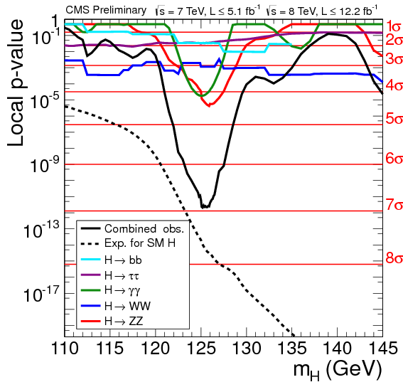
Discovery of the Higgs boson

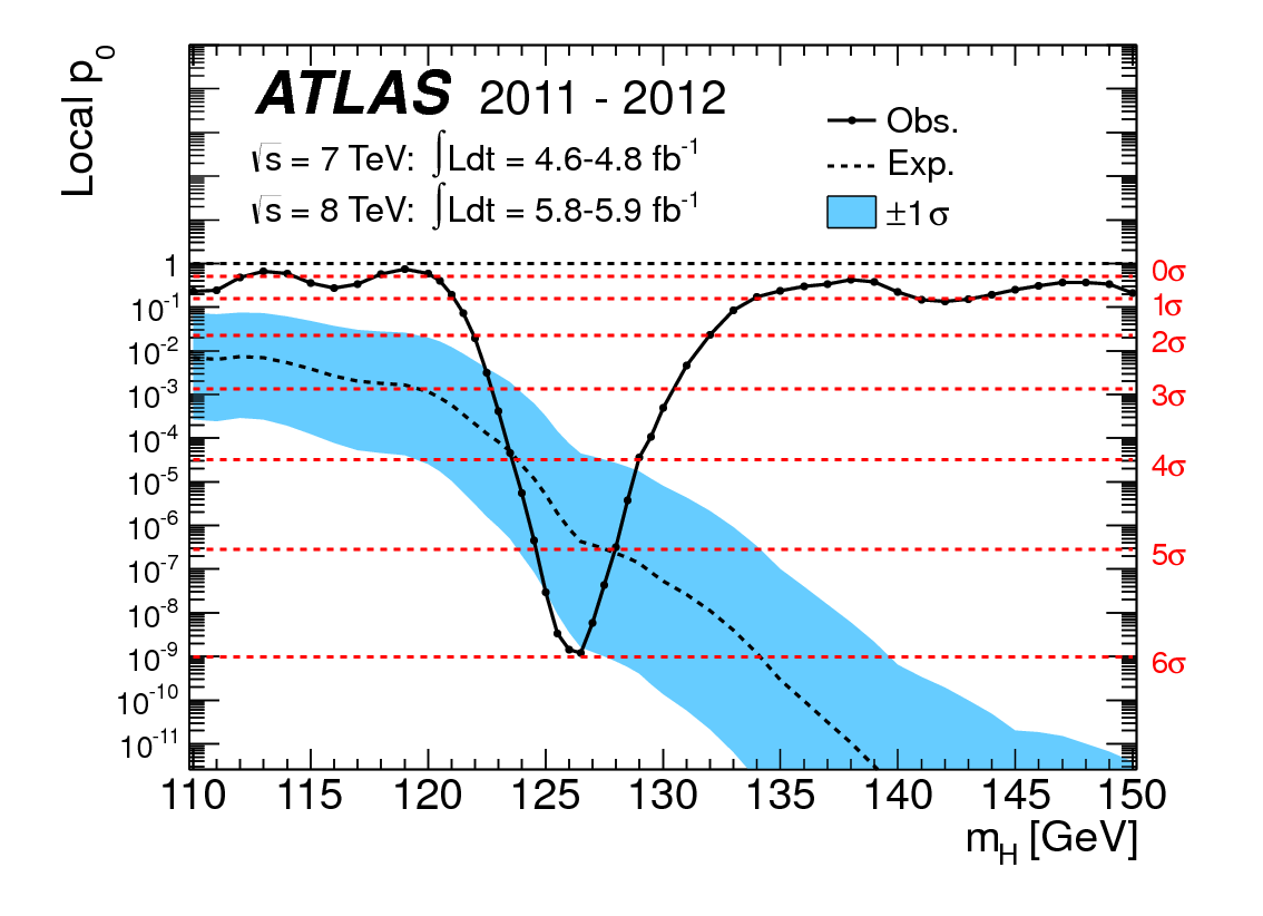
• What are
  • \(p\)-value?
  • \(\sigma\)?

Daya Bay discovery of non zero \(\theta_{13}\)

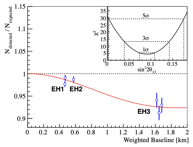
Published in: Phys.Rev.Lett. 108 (2012) 171803

• What is the oscillation fit?
  
• What is a best fit value?
  
• What is a statistical significance of the fit?

Daya Bay exclusion of parameter space for sterile neutrino

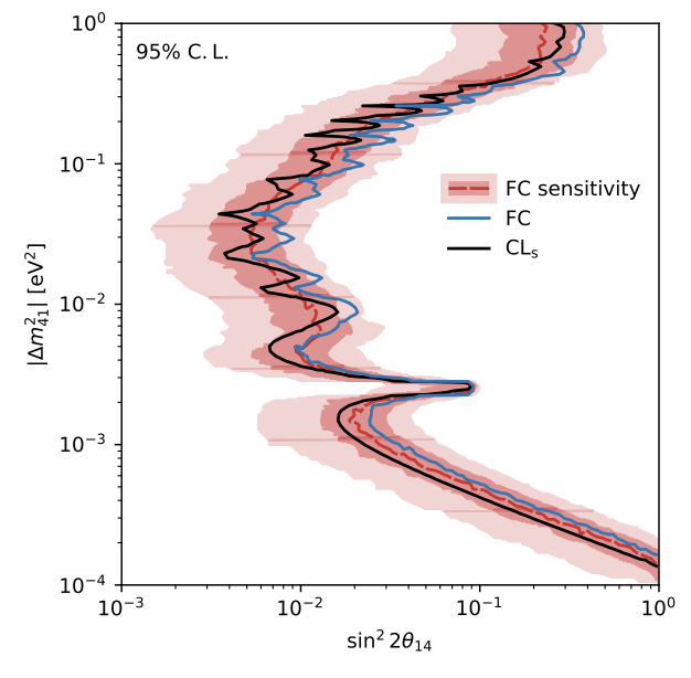
Published in: Phys.Rev.Lett. 133 (2024) 5, 051801

• What is excluded here?
  
• Why excluded?
• What is “FC sensitivity”?
  
• What is CL\(_s\)?

These figures contain many concepts

• random fluctuations
• probability distributions
• likelihood and \(\chi^2\)
• best fit
• confidence intervals and contours
• significance and \(p\)-values
• systematic uncertainties
• nuisance parameters
• profiling
• upper limits and exclusions

If you do not understand all of this — this course is for you

What will we learn?

• Probability, Bayes’ theorem
• Random variables and probability densities
• Expectation values, error propagation
• Various pdfs (probability density functions)
• The Monte Carlo method
• Statistical tests: general concepts
• Test statistics, multivariate methods
• Goodness-of-fit tests: p-values, significance, discovery and exclusion

What will we learn?

• Feldman–Cousins, CL\(_s\), and other methods
• Parameter estimation, maximum likelihood
• Method of least squares
• Interval estimation, setting limits
• Nuisance parameters, systematic uncertainties
• Examples of Bayesian approach

Let us begin

A toy example: determine the width of a Gaussian

• Assume that the data follow a Gaussian shape \[ y(x)=\exp\!\left(-\frac{x^2}{2\sigma^2}\right), \] with known center \(x_0=0\) and normalization \(N=1\).

• The only unknown parameter is the width \(\sigma\).

• We generate pseudo-data with statistical fluctuations.

• Your task is to find \(\sigma\) by comparing the model to the data.

• For each chosen value of \(\sigma\), we calculate \[ \chi^2(\sigma)=\sum_i \frac{[y_i-y(x_i;\sigma)]^2}{\delta y_i^2}. \]

• The best-fit value of \(\sigma\) minimizes \(\chi^2\).

Pseudo-data and fit

viewof sigma = Inputs.range([0.3, 2.0], {
  value: 1.0,
  step: 0.05,
  label: "trial σ"
})

viewof noise = Inputs.range([0.01, 0.15], {
  value: 0.05,
  step: 0.01,
  label: "noise δy"
})

viewof regenerate = Inputs.button("Generate new pseudo-data")

viewof overlays = {
  const control = Inputs.checkbox(
    ["show best fit", "show true σ"],
    {label: "show", value: ["show best fit"]}
  );
  control.classList.add("fit-overlays-inline");
  return control;
}

showFit = overlays.includes("show best fit")
showTruth = overlays.includes("show true σ")

// Gaussian random number
function randn() {
  const u = 1 - Math.random();
  const v = Math.random();
  return Math.sqrt(-2 * Math.log(u)) * Math.cos(2 * Math.PI * v);
}

// Fixed x values
x = Array.from({length: 21}, (_, i) => -2.5 + 0.25 * i)

// True sigma (hidden by default)
sigmaTrue = {
  regenerate;
  return 0.5 + Math.random();
}

gauss = (x, s) => Math.exp(-(x * x) / (2 * s * s))

data = {
  regenerate;
  return x.map((xi) => ({
    x: xi,
    y: gauss(xi, sigmaTrue) + noise * randn(),
    err: noise
  }));
}

chi2of = (s) => data.reduce(
  (sum, d) => sum + ((d.y - gauss(d.x, s)) / d.err) ** 2,
  0
)

chi2 = chi2of(sigma)

sigmaGrid = Array.from({length: 341}, (_, i) => 0.30 + 0.005 * i)
chi2Grid = sigmaGrid.map((s) => ({sigma: s, chi2: chi2of(s)}))
best = chi2Grid.reduce((a, b) => (a.chi2 < b.chi2 ? a : b))
sigmaFit = best.sigma
chi2min = best.chi2
ndf = Math.max(data.length - 1, 1)
dchi2 = chi2 - chi2min

trialCurve = x.map((xi) => ({x: xi, y: gauss(xi, sigma)}))
fitCurve = x.map((xi) => ({x: xi, y: gauss(xi, sigmaFit)}))
trueCurve = x.map((xi) => ({x: xi, y: gauss(xi, sigmaTrue)}))

mutable history = []
historyReset = {
  regenerate;
  mutable history = [];
  return null;
}

historyUpdate = {
  const h = history;
  const last = h.length > 0 ? h[h.length - 1] : null;
  const point = {sigma, chi2};

  if (!last || Math.abs(last.sigma - point.sigma) > 1e-9) {
    mutable history = [...h, point];
  }
  return null;
}

mainPlot = Plot.plot({
  width: 700,
  height: 380,
  x: {label: "x"},
  y: {label: "y", domain: [-0.2, 1.2]},
  grid: true,
  marks: [
    Plot.ruleX(data, {
      x: "x",
      y1: (d) => d.y - d.err,
      y2: (d) => d.y + d.err,
      stroke: "white",
      strokeWidth: 1.5
    }),
    Plot.dot(data, {x: "x", y: "y", r: 3.5, fill: "white", stroke: "white"}),
    Plot.line(trialCurve, {x: "x", y: "y", stroke: "#ff6b6b", strokeWidth: 2}),
    ...(showTruth ? [
      Plot.line(trueCurve, {
        x: "x",
        y: "y",
        stroke: "#8ec5ff",
        strokeWidth: 2,
        strokeOpacity: 0.85
      })
    ] : []),
    ...(showFit ? [
      Plot.line(fitCurve, {
        x: "x",
        y: "y",
        stroke: "#7CFC00",
        strokeWidth: 2,
        strokeDasharray: "6,4"
      })
    ] : [])
  ]
})

profilePlot = Plot.plot({
  width: 320,
  height: 230,
  x: {label: "σ", domain: [0.3, 2.0]},
  y: {label: "χ²"},
  grid: true,
  marks: [
    Plot.line(chi2Grid, {
      x: "sigma",
      y: "chi2",
      stroke: "#8ec5ff",
      strokeOpacity: 0.75
    }),
    ...(history.length > 1 ? [
      Plot.line(history, {
        x: "sigma",
        y: "chi2",
        stroke: "gray",
        strokeOpacity: 0.45
      })
    ] : []),
    Plot.dot(history.slice(0, -1), {
      x: "sigma",
      y: "chi2",
      fill: "gray",
      r: 2.8
    }),
    Plot.dot([{sigma, chi2}], {
      x: "sigma",
      y: "chi2",
      fill: "#ff6b6b",
      r: 5
    }),
    ...(showFit ? [
      Plot.dot([{sigma: sigmaFit, chi2: chi2min}], {
        x: "sigma",
        y: "chi2",
        fill: "#7CFC00",
        r: 5
      }),
      Plot.ruleY([chi2min], {
        stroke: "#7CFC00",
        strokeDasharray: "4,4"
      })
    ] : [])
  ]
})

fitStyle = html`
<style>
.fit-widget .fit-overlays-inline {
  display: flex;
  align-items: center;
  gap: 1rem;
  flex-wrap: wrap;
}

.fit-widget .fit-overlays-inline label {
  display: inline-flex;
  align-items: center;
  gap: 0.35rem;
  margin: 0;
}

.fit-widget .fit-layout {
  display: grid;
  grid-template-columns: minmax(520px, 1fr) 320px;
  gap: 1rem;
  align-items: start;
}

.fit-widget .fit-side figure {
  margin: 0;
}

@media (max-width: 980px) {
  .fit-widget .fit-layout {
    grid-template-columns: 1fr;
  }
}
</style>
`

html`
<div>
  ${fitStyle}
  <div class="fit-layout">
    <div class="fit-main">
      ${mainPlot}
    </div>
    <div class="fit-side">
      ${profilePlot}
    </div>
  </div>
  <div style="margin-top:0.8em; font-size:0.9em; line-height:1.6;">
    <div>
      <span style="color:#ff6b6b;"><b>Your choice:</b></span>
      σ = ${sigma.toFixed(2)},
      χ² = ${chi2.toFixed(2)},
      χ²/ndf = ${(chi2 / ndf).toFixed(2)}
    </div>
    ${showFit ? `
    <div>
      <span style="color:#7CFC00;"><b>Best fit:</b></span>
      σ_fit = ${sigmaFit.toFixed(3)},
      χ²_min = ${chi2min.toFixed(2)},
      Δχ² = ${dchi2.toFixed(2)}
    </div>` : ``}
    ${showTruth ? `
    <div>
      <span style="color:#8ec5ff;"><b>Truth:</b></span>
      σ_true = ${sigmaTrue.toFixed(3)}
    </div>` : ``}
  </div>
</div>
`

Exercises

Exercise

Show that the likelihood for a Poisson count \(n\) with expectation \(\mu\) is \[ L(\mu)=\frac{\mu^n e^{-\mu}}{n!}. \]