The Standard Model

The Most Successful Reconciliation of Conflicting Principles

Dmitry V. Naumov

Joint Institute for Nuclear Research

2026-07-13

What the Standard Model Is

What the Standard Model Is

• A model built in the framework of quantum field theory
  • unifies electromagnetic and weak interactions into the electroweak interaction
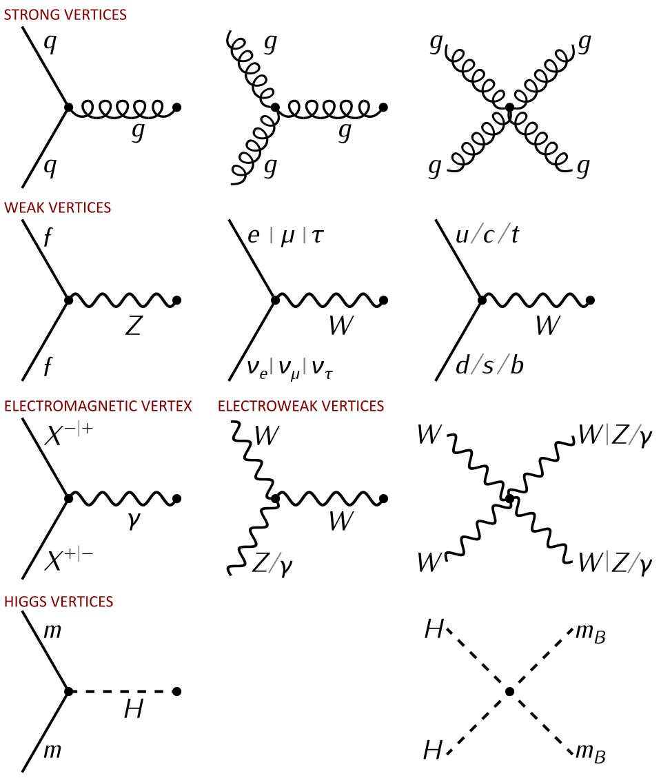
  • places electroweak and strong interactions in one gauge-theory framework
• Key nontrivial ingredients
  • local symmetries predict nontrivial interactions of quantum fields
  • spontaneous symmetry breaking turns massless fields into massive ones
  • quantum anomalies break classical conservation laws in the quantum theory
  • the Higgs field and Higgs boson were a central problem in physics for 45 years

The Code of the Universe

\[ \begin{aligned} \mathcal{L} = \sum_k\left(\overline{L}_{k,L}i\hat{D}L_{k,L}+\overline{Q}_{k,L}i\hat{D}Q_{k,L} + \sum_{\psi=\ell,\nu,u,d}\overline{\psi}_{k,R}i\hat{D}\psi_{k,R}\right) -\frac{1}{4}F_{\mu\nu}F^{\mu\nu} - \frac{1}{4}G^i_{\mu\nu}G^{i,\mu\nu} \\ + |D_{\mu}\varphi|^2-\frac{\lambda^2}{2}\left(|\varphi|^2-\frac{v^2}{2}\right)^2\\ -\sum_{k,j}\left(\lambda_{kj}^\ell\overline{L}_{k,L}\ell_{j,R}\varphi +\lambda_{kj}^\nu\overline{L}_{k,L}\nu_{j,R}\varphi_c +\lambda_{kj}^d\overline{Q}_{k,L}d_{j,R}\varphi +\lambda_{kj}^u\overline{Q}_{k,L}u_{j,R}\varphi_c+\textrm{ э.с.}\right), \end{aligned} \]

Great T-shirt print.

Easy enough?

Same Code. More Details

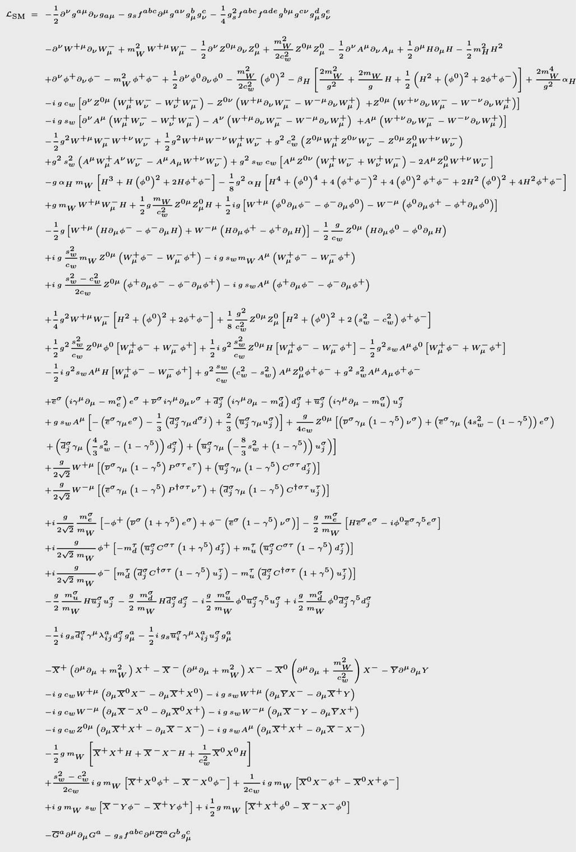
The Code of the Universe

Unity of Phenomena

The Search for the Unity of Phenomena

Maxwell’s move: two phenomena became one field.

• Electricity and magnetism stopped being separate forces.
• The electromagnetic field is one object.
• Electric and magnetic fields are different views of that object.

Old language	Unified language
electric field	electromagnetic field
magnetic field	electromagnetic field
separate phenomena	one relativistic field

Einstein’s Paradox

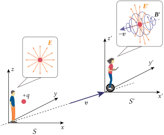
A charged particle flies past a magnet with nonzero speed \(v\).

• In the lab frame, the magnetic Lorentz force acts on it: \[ \mathbf F = q\,\mathbf v\times\mathbf B. \]
• Riding with the particle: \(v=0\).

What force acts now?

Unification of Electromagnetic and Weak Interactions

Electromagnetic and Weak Interactions Are Very Different

What to compare	Electromagnetic	Weak
Range	long range	very short range, \(\sim 10^{-18}\) m
Carrier mass	\(m_\gamma = 0\)	\(\approx 100\) GeV
Low-energy strength	strong at everyday scales	about \(10^7\)–\(10^8\) times weaker
Parity	conserves	violates
Particle identity	keeps particle type	can change particle type

Estimate the carrier mass: \[ M_W \sim \frac{g}{\sqrt{G_F}} \sim 100\ \mathrm{GeV} \]

Estimate range of the interaction: \[ R \sim \frac{1}{M_W} \sim 10^{-18}\ \mathrm{m} \]

How Do We Build Interactions with No Classical Analogy?

A Reminder: How We Built Electrodynamics

• James Clerk Maxwell created a theory of electromagnetism by unifying electricity and magnetism.

• Maxwell’s theory is incompatible with Galilean relativity but compatible with Einstein’s relativity. Thus, \[ \mathbf{E},\mathbf{B}\to A^\mu \]

• The principle of least action gives a prescription: \[ i\partial_\mu\to iD_\mu=i\partial_\mu+qA_\mu \]

• Thus, a free Lagrangian \[ \mathcal{L}=\overline{\psi}(i\gamma^\mu\partial_\mu-m)\psi \]

• becomes an interacting Lagrangian: \[ \mathcal{L}=\overline{\psi}(i\gamma^\mu D_\mu-m)\psi = \overline{\psi}(i\gamma^\mu\partial_\mu-m)\psi - q\overline{\psi}\gamma^\mu \psi A_\mu \]

The Three Physicist Friends Story

• A theorist and two experimentalists are sitting in a bar.
• The theorist says:
  • “We need to know the electron field at two astrophysically distant points. You should go there and measure it.”
  • “Remember, the phase of the electron field is a convention. You can choose it arbitrarily at each point.”
• The experimentalists fly to very distant destinations \(x\) and \(y\), with only one-way communication.

The Three Physicist Friends Story: A Problem

• The experimentalists measured the electron field at points \(x\) and \(y\) and sent the results back to the theorist.
• But they all forgot to agree on the phase convention.
• The theorist received two numbers, but he cannot compare them: \[ \psi(x)-\psi(y) \] or \[ \psi(x)e^{i\alpha(x)}-\psi(y)e^{i\alpha(y)} \]
• Not knowing which constant phases \(\alpha(x)\) and \(\alpha(y)\) were used, the theorist cannot compare the two numbers.
• The problem is even worse. For two infinitesimally close points, he cannot calculate the derivative \(\partial_\mu \psi(x)\). Therefore, even a free theory is not well-defined!

Gauge Invariance: A New Principle

• The theorist:
  • A theory should not depend on the choice of phase convention at any point.
• A free Lagrangian \[ \mathcal{L}_0=\overline{\psi}(i\gamma^\mu\partial_\mu-m)\psi \] is not invariant under local phase transformations \(\psi(x)\to e^{i\alpha(x)}\psi(x)\): \[ \mathcal{L}\to \mathcal{L} - \overline{\psi}\gamma^\mu\psi\partial_\mu\alpha(x) \]

Gauge Invariance: A New Principle

• But this Lagrangian is invariant: \[ \mathcal{L} = \overline{\psi}(i\gamma^\mu\partial_\mu-m)\psi -q\overline{\psi}\gamma^\mu\psi A_\mu-\frac{1}{4}F_{\mu\nu}F^{\mu\nu} \] under simultaneous transformations: \[ \begin{aligned} \psi(x)&\to e^{i\alpha(x)}\psi(x)\\ A_\mu(x)&\to A_\mu(x)+\frac{1}{q}\partial_\mu\alpha(x) \end{aligned} \]
• This gives QED.
• As a bonus, the photon is massless. Otherwise, \[m_A^2A_\mu A^\mu\] is not invariant under the gauge transformation.

\(X=x-x_q(t)\)

\(E_x=\dfrac{(1-\beta^2)X}{\left[X^2+(1-\beta^2)y^2\right]^{3/2}}\)

\(E_y=\dfrac{(1-\beta^2)y}{\left[X^2+(1-\beta^2)y^2\right]^{3/2}}\)

Scalar Electrodynamics as an Example of Gauge Invariance

• The same principle for a charged spin-0 field: \[ \mathcal{L}_0=(\partial_\mu\phi^*)(\partial^\mu\phi)-m^2\phi^*\phi-\frac{1}{4}F_{\mu\nu}F^{\mu\nu}. \]

• Make the theory gauge invariant by replacing \(\partial_\mu\to D_\mu\): \[ \begin{aligned} D_\mu&=\partial_\mu+iqA_\mu,\\ \mathcal{L}&=(D_\mu\phi)^*(D^\mu\phi)-m^2\phi^*\phi-\frac{1}{4}F_{\mu\nu}F^{\mu\nu}. \end{aligned} \]

• Expanding the covariant derivatives gives \[ \begin{aligned} \mathcal{L}=\mathcal{L}_0 &-iqA^\mu\phi^*(\partial_\mu\phi) +iq(\partial_\mu\phi^*)A^\mu\phi\\ &+q^2\phi^*\phi A^\mu A_\mu . \end{aligned} \]

• Gauge invariance predicts the interaction between \(\phi\) and \(A_\mu\)!

Big Cats Need a Break

\(\displaystyle \left(i\gamma^\mu\partial_\mu-m\right)\psi=0\)

\(\displaystyle \left(\Box+m^2\right)\phi=0\)

\(\displaystyle \partial_\mu F^{\mu\nu}+m^2A^\nu=0\)

\(\displaystyle \left(\Box+m^2\right)G(x)=\delta^{(4)}(x)\)

\(\displaystyle \mathcal{L}_{\mathrm{int}}=-e\,\bar{\psi}\gamma^\mu\psi A_\mu\)

\(\displaystyle \mathcal{L}_{\mathrm{SM}}=\sum_\psi\bar{\psi}i\gamma^\mu D_\mu\psi+|D_\mu\phi|^2-V(\phi)+\cdots\)

\(\displaystyle \mathcal{L}_{\mathrm{QCD}}=-\frac14G^a_{\mu\nu}G^{a\mu\nu}+\bar{q}\,i\gamma^\mu D_\mu q\)

\(\displaystyle W[C]=\operatorname{P}\exp\!\left(ig\oint_C A_\mu dx^\mu\right)\)

\(\displaystyle \partial_\mu J_5^\mu=\frac{g^2}{16\pi^2}F_{\mu\nu}\widetilde{F}^{\mu\nu}\)

\(\displaystyle \tau_{\pi^0}=8.4\times10^{-17}\,\mathrm{s}\)

\(\displaystyle V(\phi)=\lambda\left(|\phi|^2-\frac{v^2}{2}\right)^2\)

\(\displaystyle P(\nu_\mu\to\nu_e)=\sin^2 2\theta\,\sin^2\!\frac{\Delta m^2L}{4E}\)

\(\displaystyle D_\mu=\partial_\mu+igA_\mu^aT^a\)

The Algorithm

• Gauge invariance is now a method for predicting interactions.
• The algorithm is simple:
  • Take a free theory.
  • Replace \(\partial_\mu\to D_\mu\)
  • Introduce one compensating field \(A^\mu_i\) for each generator of the symmetry group.
  • Introduce \(F_{\mu\nu}\) and a gauge-invariant Lagrangian for the new fields.
  • The interaction is no longer optional.

Symmetry Becomes Dynamics

If symmetries give conservation laws, perhaps interactions are also dictated by symmetry.

Salam and Ward, 1961

The Pillars of the Standard Model

1. A symmetry group \[ SU(2)_L\times U(1)_Y \]

• it requires all fermion and gauge-boson masses to vanish. This is not what we observe.

2. A symmetry breaking mechanism

• it gives particles their masses

Origin of Mass

Six Definitions of Mass

1. Inertial mass — a measure of resistance to acceleration under an applied force.
2. Active gravitational mass — the strength of the gravitational field produced by a body.
3. Passive gravitational mass — a measure of response to an external gravitational field.
4. Rest energy — defined through the relation \(E=mc^2\).
5. Source of spacetime curvature — the role of mass in general relativity.
6. Quantum mass — a quantity inverse to the Compton wavelength.

Experiments show that all these masses are equal to, or proportional to, one another.

The Secret Origin of Mass

• Modern physics suggests that masses appeared dynamically shortly after the Big Bang, through a phase transition.
• After the phase transition, a scalar (Higgs) field condensed; this generated particle masses.
• Metaphorically, we live inside a superconductor.
• There are two distinct mechanisms of mass generation:
  • for gauge bosons
  • for fermions.

Mass Generation of a Vector Boson

Meissner Effect

• An external magnetic field is expelled from a superconductor.
• Near the surface it induces a superconducting current.
• This screening current produces the levitation force.
• In field language: \[ \left(\nabla^2-m_\gamma^2\right)A^\mu=0, \qquad m_\gamma^2=\frac{q^2n_e}{m}. \]

\[ \nabla^2\mathbf B=\lambda_L^{-2}\mathbf B,\qquad \lambda_L=\sqrt{\frac{m}{\mu_0 n_s q^2}} \]

\[ \mathbf B(x)=\mathbf B_0 e^{-x/\lambda_L},\qquad \nabla\times\mathbf J_s=-\frac{1}{\mu_0\lambda_L^2}\mathbf B \]

\[ U_B=\int\frac{B^2}{2\mu_0}\,dV,\qquad F_z=-\frac{\partial U_B}{\partial z} \]

\[ p_B=\frac{B^2}{2\mu_0},\qquad F_z=mg \]

The Higgs Mechanism in the Standard Model

• The Higgs scalar field produces a screening current: \[ j^\mu = -e^2 v^2 A^\mu \]
• The Maxwell equation \[ \partial_\nu F^{\nu\mu} = j^\mu =-e^2 v^2 A^\mu \] yields \[ \left(\partial^2+m_A^2\right)A^\mu=0, \quad \mathrm{with}\quad \boxed{m_A^2= e^2v^2}. \]
• This is exactly the Meissner effect.

Mass Generation of a Fermion

Two Coupled Pendulums

• Small angles: \[ \ddot{\boldsymbol{\theta}}=-D\boldsymbol{\theta}, \qquad \boldsymbol{\theta}= \begin{pmatrix} \theta_1 \\ \theta_2 \end{pmatrix} \] \[ D= \begin{pmatrix} \omega_0^2+\frac{k}{m_1} & -\frac{k}{m_1}\\ -\frac{k}{m_2} & \omega_0^2+\frac{k}{m_2} \end{pmatrix}, \] \[ \omega_0^2=\frac{g}{L}. \]
• Normal modes: \[ \omega_-^2=\omega_0^2, \qquad \boldsymbol v_-=(1,1) \] \[ \omega_+^2=\omega_0^2+ k\left(\frac{1}{m_1}+\frac{1}{m_2}\right), \qquad \boldsymbol v_+= \left(1,-\frac{m_1}{m_2}\right) \]

Chiral Waves Become Massive Normal Modes

• In 1D, with \(c=\hbar=1\), massless chiral waves are independent: \[ i\partial_t \begin{pmatrix}R\\L\end{pmatrix} = \begin{pmatrix}p&0\\0&-p\end{pmatrix} \begin{pmatrix}R\\L\end{pmatrix}. \]

• The Higgs condensate couples them: \[ m=\frac{y_f v}{\sqrt2}, \qquad H(p)= \begin{pmatrix}p&m\\m&-p\end{pmatrix}. \]
• Normal frequencies: \[ \omega_\pm(p)=\pm\sqrt{p^2+m^2}. \]
• At rest: \[ \Psi_+(0)=\frac{R+L}{\sqrt2}, \qquad \Psi_-(0)=\frac{R-L}{\sqrt2}. \]

A Finite Condensate Layer

• Let the Higgs condensate occupy a layer: \[ m(x)= \begin{cases} 0, & x<0,\\ m_0, & 0<x<a,\\ 0, & x>a. \end{cases} \]
• For \(E>m_0\), the static layer conserves \(E\): \[ E^2=q^2+m_0^2, \qquad q=\sqrt{E^2-m_0^2}<E, \qquad v_g=\frac{q}{E}<1. \]
• For an incoming \(R\) wave: \[ r= \frac{-im_0\sin qa} {q\cos qa-iE\sin qa}, \] \[ t= \frac{q\,e^{-iEa}} {q\cos qa-iE\sin qa}. \]
• The slider changes \(a\) in the exact solution.

condensate width m₀a = 3.20

Two Mechanisms, One Condensate

The Higgs condensate creates a gap in the spectrum in two different ways.

Vector bosons: Meissner mechanism

• The condensate behaves like a superconductor.
• A gauge field induces a screening current.
• Free propagation is lost: the field becomes short-range. \[ \left(\partial^2+m_A^2\right)A^\mu=0, \qquad m_A^2=e^2v^2. \]

Fermions: coupled chiral waves

• Without the condensate, \(R\) and \(L\) move independently at \(c\).
• The condensate couples them: left sources right, and right sources left. \[ m_f=\frac{y_fv}{\sqrt2}. \]
• Stable waves are normal modes: \[ \Psi_\pm(0)=\frac{R\pm L}{\sqrt2}. \]

Neutron Decay in QFT

The Code Runs

principle

local gauge symmetry

interactions are forced by local phase freedom

\(D_\mu=\partial_\mu+igA_\mu\)

condensate

spontaneous symmetry breaking

weak carriers become massive

\(M_W=\dfrac{gv}{2}\)

coupling

chiral fermions meet the Higgs field

left and right become massive normal modes

\(m_f=\dfrac{y_fv}{\sqrt2}\)

⇒

observable process

\(n\rightarrow p+e^-+\bar\nu_e\)

weak vertex, massive particles, chiral structure, one calculable quantum amplitude

The Standard Model is not a list of particles. It is a consistency machine.