Masterclass 1: Fluxes, Event Rates, and a Normalization Fit

SK-like event spectrum from solar \(^8\mathrm{B}\) neutrinos

Dmitry V. Naumov

JINR

2026-06-01

Lesson Map

• Tasks
• Inputs
• Event Model
• Pseudo-Data and Fit
• What to Study
• Homework

Tasks

Goal for This Session

Build the first quantitative model for an SK-like solar-neutrino measurement:

\[ {}^8\mathrm{B}\ \nu_e \to \nu e\ \mathrm{scattering} \to e^-_{\rm recoil}. \]

Today we compute:

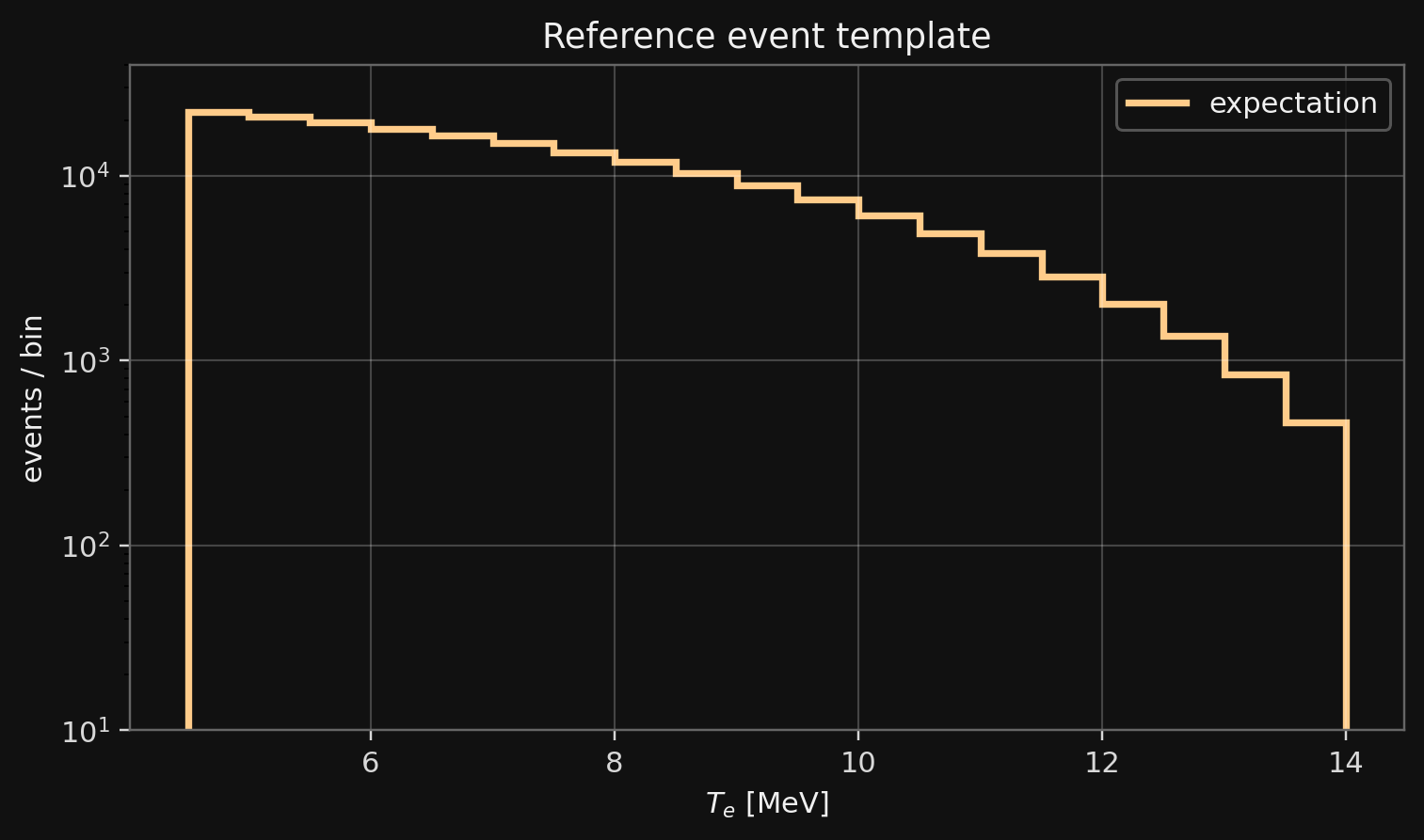
• expected event counts in recoil-electron energy bins;
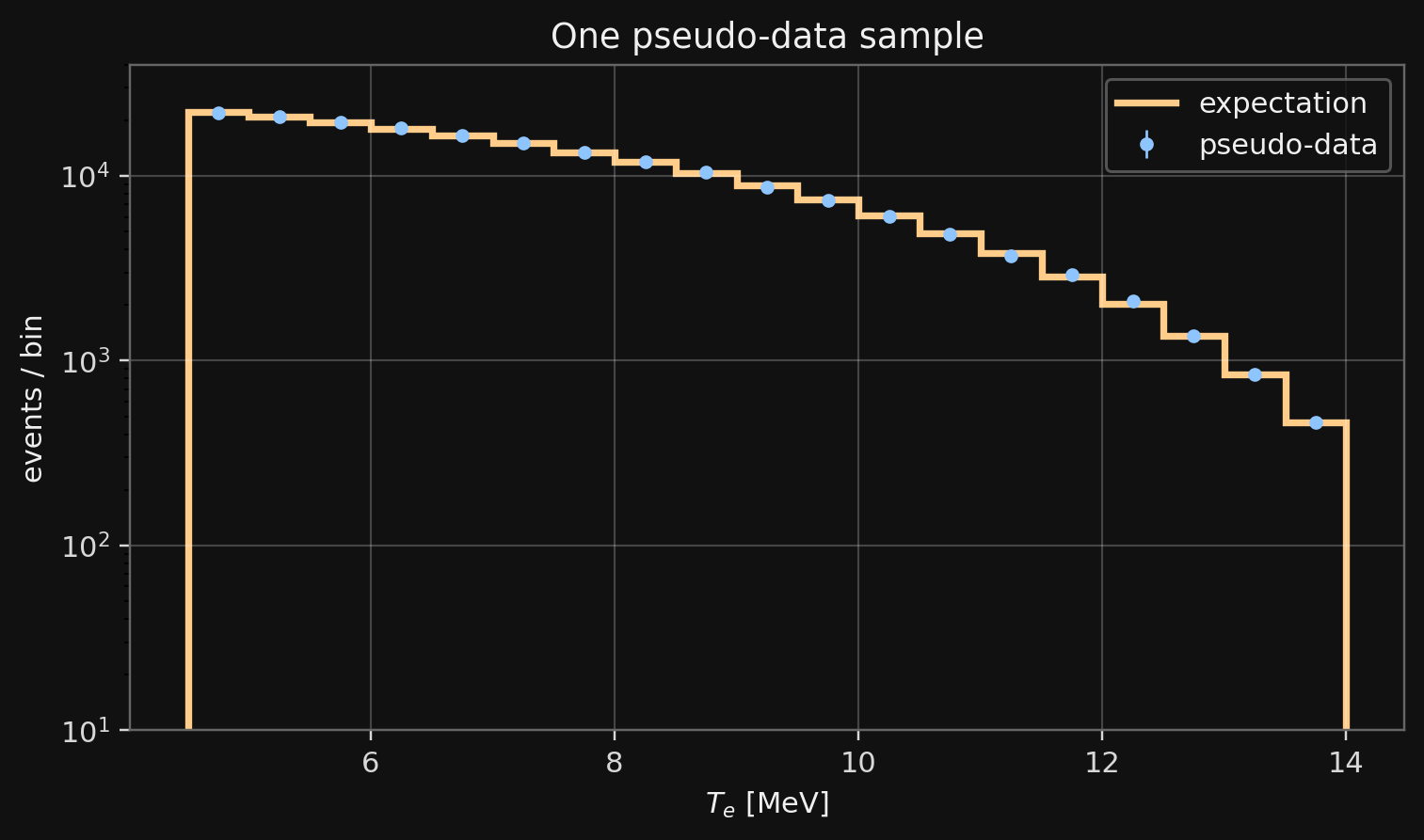
• pseudo-data from those expected counts;
• a one-parameter fit of the \(^8\mathrm{B}\) flux normalization.

Fit Parameter

Use one free parameter:

\[ \Phi_{^8\mathrm{B}} \to \alpha_B\,\Phi_{^8\mathrm{B}}. \]

The first-session fit is

\[ \alpha_B = 1 \quad\hbox{for the reference input flux.} \]

Oscillations are not fitted today:

\[ P_{ee}=1. \]

Main Output

The notebook must produce:

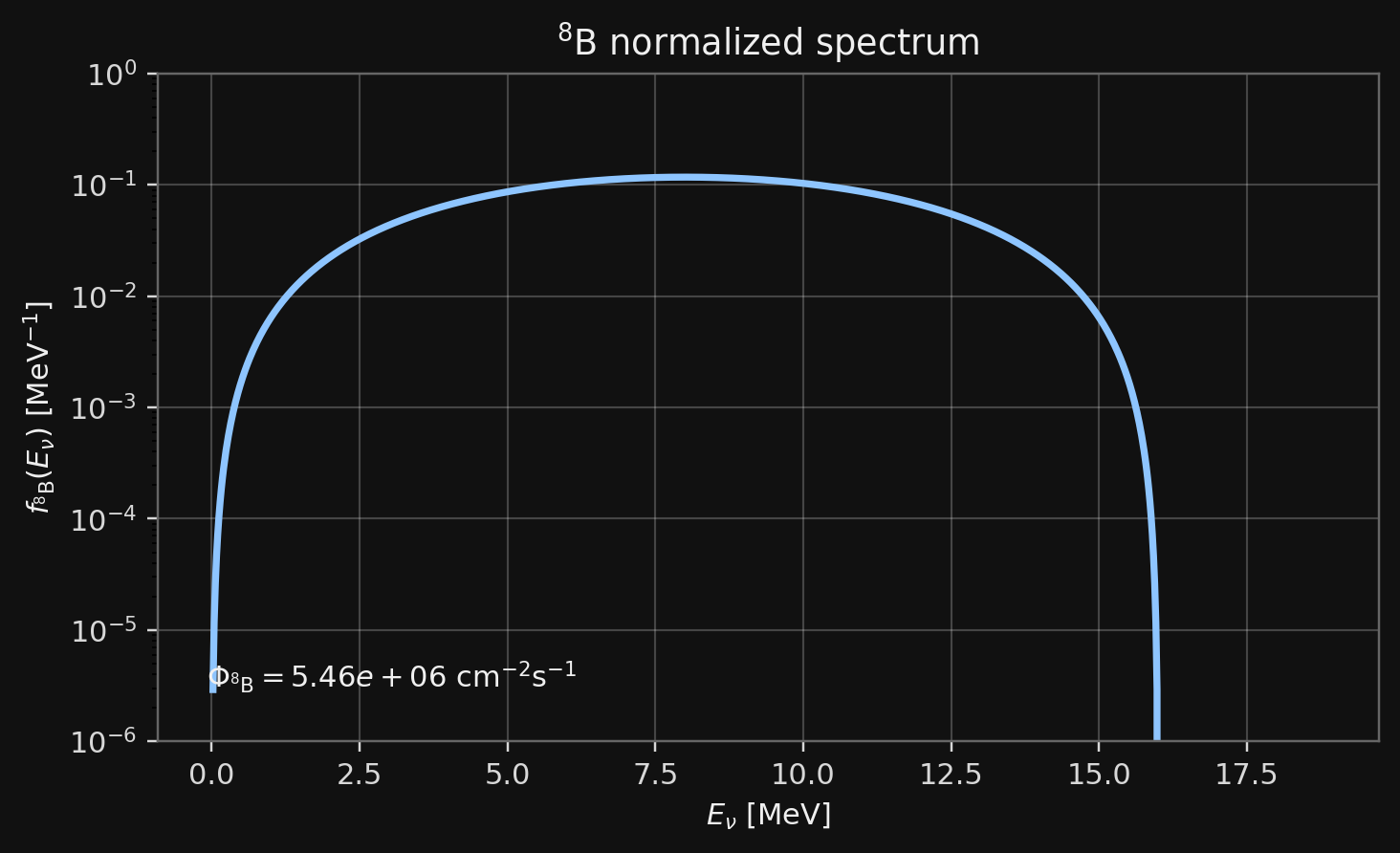
• \(^8\mathrm{B}\) neutrino spectrum;
• SK-like recoil spectrum \(dN/dT_e\);
• event total above a chosen threshold;
• pseudo-data in the same bins;
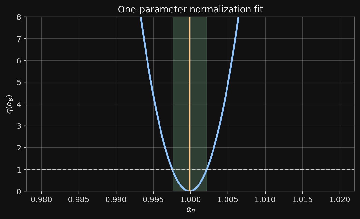
• \(\hat\alpha_B\) and a one-dimensional interval from \(q(\alpha_B)\).

Inputs

Project Page

Project page:

https://neutrinohit.github.io/neutrinophysics/
solar-neutrino-masterclass/

Tables used today:

data/masterclass1/solar_fluxes.csv
data/masterclass1/energy_spectra.csv
data/masterclass1/nu_electron_recoil_cross_sections.csv

Load the Tables

From the web page:

import numpy as np
import pandas as pd

BASE = "https://neutrinohit.github.io/neutrinophysics/solar-neutrino-masterclass"

fluxes = pd.read_csv(f"{BASE}/data/masterclass1/solar_fluxes.csv")
spectra = pd.read_csv(f"{BASE}/data/masterclass1/energy_spectra.csv")
xs = pd.read_csv(f"{BASE}/data/masterclass1/nu_electron_recoil_cross_sections.csv")

For a local notebook, replace BASE by the local project directory.

Select \(^8\mathrm{B}\)

phi_b8 = float(
    fluxes.loc[fluxes["source"] == "B8", "flux_cm2_s"].iloc[0]
)

b8 = spectra.loc[spectra["source"] == "B8"].copy()
b8 = b8.sort_values("E_MeV")

Here

\[ \Phi_{^8\mathrm{B}}=\int dE_\nu\,\frac{d\Phi_{^8\mathrm{B}}}{dE_\nu}, \qquad \frac{d\Phi_{^8\mathrm{B}}}{dE_\nu} = \Phi_{^8\mathrm{B}} f_{^8\mathrm{B}}(E_\nu). \]

The table column spectrum_per_MeV is \(f_{^8\mathrm{B}}(E_\nu)\).

Expected check:

Phi_B8 = 5.460000e+06 cm^-2 s^-1

Check the Spectrum

Check the normalization:

norm = np.trapezoid(b8["spectrum_per_MeV"], b8["E_MeV"])
print(norm)

Expected output:

1.000000000000

Plot:

ax = b8.plot(
    x="E_MeV",
    y="spectrum_per_MeV",
    logy=True,
    legend=False
)
ax.set_xlabel(r"$E_\nu$ [MeV]")
ax.set_ylabel(r"$f_{^8\mathrm{B}}(E_\nu)$ [MeV$^{-1}$]")

Event Model

Target Electrons

For water,

\[ N_e = 10 N_A\frac{M_{\rm water}}{18~\mathrm{g}}. \]

For an exposure written as \(M_{\rm water}T_{\rm live}\),

\[ N_eT_{\rm live} = 10N_A\frac{M_{\rm water}}{18~\mathrm{g}}T_{\rm live}. \]

The CSV units are practical units: flux in \(\mathrm{cm^{-2}s^{-1}}\), cross section in \(\mathrm{cm^2\,MeV^{-1}}\).

Target Electrons

Use in the example:

N_A = 6.02214076e23
seconds_per_year = 365.25 * 24 * 3600

mass_g = 100.0e9          # 100 kton water
T_live = seconds_per_year # one year
N_e = 10.0 * N_A * mass_g / 18.0

Expected check:

N_e = 3.345634e+34

Binned Prediction

For recoil-energy bin \(j\),

\[ \mu_j(\alpha_B) = \alpha_B\,N_eT_{\rm live} \int_{T_j}^{T_{j+1}}dT_e \int dE_\nu\, \Phi_{^8\mathrm{B}}f_{^8\mathrm{B}}(E_\nu) \frac{d\sigma_{\nu_e e}(E_\nu,T_e)}{dT_e}. \]

Today:

\[ \mu_j(\alpha_B)=\alpha_B\,m_j. \]

The fixed template \(m_j\) is the reference prediction for \(\alpha_B=1\).

Cross-Section Table

Required columns:

E_MeV
T_e_MeV
dsigma_nue_cm2_per_MeV

Use interpolation for the \(^8\mathrm{B}\) spectral shape:

shape = np.interp(
    xs["E_MeV"],
    b8["E_MeV"],
    b8["spectrum_per_MeV"],
    left=0.0,
    right=0.0,
)

xs = xs.assign(dphi_dE=phi_b8 * shape)

Expected checks:

cross-section grid = 188 x 181
dE = 0.100267 MeV, dT = 0.100000 MeV

Tabular Integral

For each table row \((E_\nu^a,T_e^b)\), define a weight

\[ w_{ab} = N_eT_{\rm live} \Phi_{^8\mathrm{B}}f_{^8\mathrm{B}}(E_\nu^a) \frac{d\sigma_{\nu_e e}(E_\nu^a,T_e^b)}{dT_e} \Delta E_\nu\Delta T_e . \]

Then the prediction in recoil bin \(j\) is

\[ m_j \simeq \sum_{a,b:\,T_e^b\in [T_j,T_{j+1})} w_{ab}. \]

First compute row weights. Then assign rows to recoil-energy bins.

Event Template

E_grid = np.sort(xs["E_MeV"].unique())
T_grid = np.sort(xs["T_e_MeV"].unique())
dE = np.median(np.diff(E_grid))
dT = np.median(np.diff(T_grid))

Event Template

Tmin, Tmax, bin_width = 4.5, 14.0, 0.5
edges = np.arange(Tmin, Tmax + 0.5 * bin_width, bin_width)
nbins = len(edges) - 1
bin_id = np.digitize(xs["T_e_MeV"], edges) - 1

valid = (0 <= bin_id) & (bin_id < nbins)
integrand = (
    N_e * T_live
    * xs["dphi_dE"]
    * xs["dsigma_nue_cm2_per_MeV"]
    * dE * dT
)

m = np.bincount(bin_id[valid], weights=integrand[valid], minlength=nbins)
centers = 0.5 * (edges[:-1] + edges[1:])

Plot the Prediction

import matplotlib.pyplot as plt

plt.stairs(m, edges)
plt.xlabel(r"$T_e$ [MeV]")
plt.ylabel("expected events / bin")
plt.yscale("log")
plt.show()

Expected first bins:

T_low  T_high  events
4.5    5.0     22174.6
5.0    5.5     20898.3
5.5    6.0     19528.7

Useful checks:

• \(m_j\ge 0\);
• \(\sum_j m_j\) decreases when \(T_{\min}\) increases;

• changing nbins should not change \(\sum_j m_j\) much.

Pseudo-Data and Fit

Generate Pseudo-Data

Choose a true normalization:

\[ \alpha_B^{\rm true}=1. \]

Generate counts:

rng = np.random.default_rng(12345)
alpha_true = 1.0
n = rng.poisson(alpha_true * m)
print(m.sum(), n.sum())

Plot data and expectation in the same bins.

Expected output for this seed:

186693.543 186665

Likelihood

For Poisson bins,

\[ \ell(\alpha_B) = \sum_j \left[ n_j\ln\mu_j(\alpha_B)-\mu_j(\alpha_B) \right] +\mathrm{const}. \]

Use

\[ q(\alpha_B) = -2\left[\ell(\alpha_B)-\ell(\hat\alpha_B)\right]. \]

For one fitted parameter, the usual \(1\sigma\) interval is given by

\[ q(\alpha_B)=1. \]

Equivalently, the one-dimensional \(1\sigma\) contour is

\[ q(\alpha_B)\le 1. \]

Grid Fit

alphas = np.linspace(0.98, 1.02, 401)
mu = alphas[:, None] * m[None, :]
mu = np.maximum(mu, 1e-300)

ll = np.sum(n[None, :] * np.log(mu) - mu, axis=1)
q = -2.0 * (ll - ll.max())

alpha_hat = alphas[np.argmax(ll)]
print(alpha_hat)

Plot \(q(\alpha_B)\) and mark \(q=1\).

Expected output:

alpha_hat = 0.9998
q <= 1 interval: 0.99760 ... 1.00210

Analytic Check

Because this first model is linear,

\[ \mu_j(\alpha_B)=\alpha_B m_j, \]

the maximum-likelihood estimator is

\[ \hat\alpha_B = \frac{\sum_j n_j}{\sum_j m_j}. \]

Use this as a check of the grid fit:

alpha_hat_check = n.sum() / m.sum()
print(alpha_hat, alpha_hat_check)

Expected output:

0.9998 0.999847

What to Study

Threshold Sensitivity

Repeat the fit for several thresholds:

\[ T_{\min}=3,\ 4.5,\ 6~\mathrm{MeV}. \]

For each threshold report:

• total expected events \(\sum_j m_j\);
• best fit \(\hat\alpha_B\);
• approximate \(1\sigma\) interval;
• whether the result is stable against binning changes.

Threshold Sensitivity

Expected reference table for 100 kton year:

Tmin [MeV]  bins  expected events  stat. scale
3.0         22    259784.969       0.001962
4.5         19    186693.543       0.002314
6.0         16    124092.018       0.002839

Numerical Stability

Change:

• number of recoil-energy bins;
• upper endpoint \(T_{\max}\);
• threshold \(T_{\min}\);
• random seed for pseudo-data.

The fitted value moves because the pseudo-data change. The expected uncertainty should scale roughly as

\[ \sigma_{\alpha_B}\sim\frac{1}{\sqrt{\sum_j m_j}}. \]

Homework

Computational Part

Submit a notebook with:

1. Plot of \(f_{^8\mathrm{B}}(E_\nu)\) and \(d\Phi_{^8\mathrm{B}}/dE_\nu\).
2. SK-like recoil spectrum \(m_j\) for \(T_{\min}=4.5~\mathrm{MeV}\).
3. Table of total expected events for \(T_{\min}=3,\ 4.5,\ 6~\mathrm{MeV}\).
4. One pseudo-data sample.
5. Fit of \(\alpha_B\): \(\hat\alpha_B\), \(q(\alpha_B)\), and the \(1\sigma\) interval.
6. A short check comparing the grid fit with \(\hat\alpha_B=\sum n_j/\sum m_j\).

Theory Part

Study the Gamow window for:

\[ p+p,\qquad {}^3\mathrm{He}+{}^4\mathrm{He},\qquad {}^7\mathrm{Be}+p. \]

For each reaction estimate \(E_0\) at a solar-core temperature and compare the scales.

Theory Part

Study the astrophysical \(S\)-factor.

Choose one solar reaction and summarize:

• which experimental measurements exist;
• what energy range they cover;
• how far the extrapolation to solar energies is;
• what dominates the uncertainty.

The result should be a short critical note, not a list of references.

Advanced Part

Derive or verify the \(\nu e\) differential cross section from QFT:

\[ \nu_\ell + e^- \to \nu_\ell + e^-. \]

Answer explicitly:

Why is the \(\nu_e e\) cross section larger than the \(\nu_\mu e\) and \(\nu_\tau e\) cross sections?

Optional Extensions

Good extensions after the first session:

• expected sensitivity to \(\alpha_B\) as a function of threshold;
• binning stability of the event integral;
• comparison of \(\nu_e e\) and \(\nu_x e\) event templates;
• compute the expected event contribution of each solar-neutrino source as a function of the recoil-electron threshold.