solarFitEventsInput = Inputs.range([5000, 120000], {value: 60000, step: 1000, label: "N₀"})
solarFitS12TrueInput = Inputs.range([0.20, 0.42], {value: 0.307, step: 0.002, label: "true sin²θ₁₂"})
solarFitDmTrueInput = Inputs.range([5.0, 10.0], {value: 7.42, step: 0.05, label: "true Δm²₂₁"})
solarFitNBinsInput = Inputs.range([8, 28], {value: 18, step: 1, label: "bins"})
solarFitThresholdInput = Inputs.range([3.0, 7.0], {value: 3.0, step: 0.25, label: "Tₑ,min [MeV]"})
solarFitRegenerateInput = Inputs.button("new pseudo-data", {value: 0, reduce: () => Date.now()})

solarFitEvents = Generators.input(solarFitEventsInput)
solarFitS12True = Generators.input(solarFitS12TrueInput)
solarFitDmTrue = Generators.input(solarFitDmTrueInput)
solarFitNBins = Generators.input(solarFitNBinsInput)
solarFitThreshold = Generators.input(solarFitThresholdInput)
solarFitRegenerate = Generators.input(solarFitRegenerateInput)

solarFitB8Rows = FileAttachment("../data/b8_spectrum.csv").csv({typed: true})
solarFitCrossRows = FileAttachment("../data/masterclass1/nu_electron_recoil_cross_sections.csv").csv({typed: true})

solarFitB8Table = solarFitB8Rows
  .map(row => ({E: Number(row.E_MeV), shape: Number(row.shape)}))
  .sort((a, b) => a.E - b.E)

solarFitB8ShapeAt = E => {
  if (E < solarFitB8Table[0].E || E > solarFitB8Table[solarFitB8Table.length - 1].E) return 0;
  let lo = 0;
  let hi = solarFitB8Table.length - 1;
  while (hi - lo > 1) {
    const mid = Math.floor((lo + hi) / 2);
    if (solarFitB8Table[mid].E <= E) lo = mid;
    else hi = mid;
  }
  const a = solarFitB8Table[lo];
  const b = solarFitB8Table[hi];
  const f = (E - a.E) / Math.max(b.E - a.E, 1e-12);
  return a.shape + f * (b.shape - a.shape);
}

solarFitTGrid = Array.from({length: solarFitNBins}, (_, i) => {
  const low = solarFitThreshold;
  const high = 14.0;
  const t1 = low + i * (high - low) / solarFitNBins;
  const t2 = low + (i + 1) * (high - low) / solarFitNBins;
  return {i, t1, t2, t: 0.5 * (t1 + t2), groups: new Map()};
})

solarFitBinWeights = {
  const dE = 0.05;
  const dT = 0.10;
  const tLow = solarFitTGrid[0].t1;
  const tHigh = solarFitTGrid[solarFitTGrid.length - 1].t2;
  for (const row of solarFitCrossRows) {
    const E = Number(row.E_MeV);
    const T = Number(row.T_e_MeV);
    if (E < 0.05 || E > 16.0) continue;
    if (T + 0.5 * dT <= tLow || T - 0.5 * dT >= tHigh) continue;
    const shape = solarFitB8ShapeAt(E);
    if (!(shape > 0)) continue;
    const dsE = Number(row.dsigma_nue_cm2_per_MeV);
    const dsX = Number(row.dsigma_nux_cm2_per_MeV);
    if (!(dsE > 0) && !(dsX > 0)) continue;
    const cellLow = Math.max(tLow, T - 0.5 * dT);
    const cellHigh = Math.min(tHigh, T + 0.5 * dT);
    if (cellHigh <= cellLow) continue;
    const firstBin = Math.max(0, Math.floor((cellLow - tLow) / (tHigh - tLow) * solarFitTGrid.length));
    const lastBin = Math.min(
      solarFitTGrid.length - 1,
      Math.floor((cellHigh - 1e-12 - tLow) / (tHigh - tLow) * solarFitTGrid.length)
    );
    for (let ibin = firstBin; ibin <= lastBin; ++ibin) {
      const bin = solarFitTGrid[ibin];
      const overlap = Math.max(0, Math.min(cellHigh, bin.t2) - Math.max(cellLow, bin.t1));
      if (!(overlap > 0)) continue;
      const key = E.toFixed(2);
      const group = bin.groups.get(key) ?? {E, sigmaE: 0, sigmaX: 0};
      group.sigmaE += shape * dsE * dE * overlap;
      group.sigmaX += shape * dsX * dE * overlap;
      bin.groups.set(key, group);
    }
  }
  return solarFitTGrid.map(bin => ({
    i: bin.i,
    t1: bin.t1,
    t2: bin.t2,
    t: bin.t,
    weights: Array.from(bin.groups.values())
  }));
}

solarFitPee = (Emev, s12, dmMicro) => {
  const gfEv = 1.1663787e-23;
  const cmToEvInv = 5.067730716e4;
  const cmMinus3ToEv3 = 1 / Math.pow(cmToEvInv, 3);
  const neCore = 6.0e25;
  const ve = Math.SQRT2 * gfEv * neCore * cmMinus3ToEv3;
  const dm2 = dmMicro * 1e-5;
  const c2 = 1 - 2 * s12;
  const s22 = 4 * s12 * (1 - s12);
  const a = 2 * Emev * 1e6 * ve / dm2;
  const cos2ThetaM = (c2 - a) / Math.sqrt((c2 - a) * (c2 - a) + s22);
  return Math.min(0.98, Math.max(0.02, 0.5 + 0.5 * c2 * cos2ThetaM));
}

solarFitExpectedRaw = (s12, dmMicro) => solarFitBinWeights.map(bin => {
  let mu = 0;
  for (const row of bin.weights) {
    const pee = solarFitPee(row.E, s12, dmMicro);
    mu += pee * row.sigmaE + (1 - pee) * row.sigmaX;
  }
  return mu;
})

solarFitNoOscRaw = solarFitBinWeights.map(bin =>
  bin.weights.reduce((sum, row) => sum + row.sigmaE, 0)
)

solarFitNoOscTotalRaw = solarFitNoOscRaw.reduce((sum, x) => sum + x, 0)

solarFitExpected = (s12, dmMicro) => {
  const raw = solarFitExpectedRaw(s12, dmMicro);
  const scale = solarFitEvents / Math.max(solarFitNoOscTotalRaw, 1e-300);
  return raw.map(x => x * scale);
}

solarFitNoOscExpected = solarFitNoOscRaw.map(x => x * solarFitEvents / Math.max(solarFitNoOscTotalRaw, 1e-300))

solarFitRandn = () => {
  const u1 = Math.max(Math.random(), 1e-12);
  const u2 = Math.random();
  return Math.sqrt(-2 * Math.log(u1)) * Math.cos(2 * Math.PI * u2);
}

solarFitPoisson = lambda => {
  if (lambda <= 0) return 0;
  if (lambda > 80) return Math.max(0, Math.round(lambda + Math.sqrt(lambda) * solarFitRandn()));
  const limit = Math.exp(-lambda);
  let k = 0;
  let product = 1;
  do {
    ++k;
    product *= Math.random();
  } while (product > limit);
  return k - 1;
}

solarFitData = {
  solarFitRegenerate;
  const mu = solarFitExpected(solarFitS12True, solarFitDmTrue);
  return solarFitBinWeights.map((bin, i) => ({
    ...bin,
    n: solarFitPoisson(mu[i]),
    muTrue: mu[i],
    muNoOsc: solarFitNoOscExpected[i]
  }));
}

solarFitLogLike = (s12, dmMicro) => {
  const mu = solarFitExpected(s12, dmMicro);
  let ll = 0;
  for (let i = 0; i < solarFitData.length; ++i) {
    const lambda = Math.max(mu[i], 1e-12);
    ll += solarFitData[i].n * Math.log(lambda) - lambda;
  }
  return ll;
}

solarFitS12Grid = Array.from({length: 61}, (_, i) => 0.20 + i * (0.42 - 0.20) / 60)
solarFitDmGrid = Array.from({length: 61}, (_, i) => 5.0 + i * (10.0 - 5.0) / 60)

solarFitResult = {
  const rows = [];
  let best = {s12: 0, dm: 0, ll: -Infinity};
  for (let ia = 0; ia < solarFitS12Grid.length; ++ia) {
    const s12 = solarFitS12Grid[ia];
    for (let id = 0; id < solarFitDmGrid.length; ++id) {
      const dm = solarFitDmGrid[id];
      const ll = solarFitLogLike(s12, dm);
      rows.push({ia, id, s12, dm, ll});
      if (ll > best.ll) best = {s12, dm, ll};
    }
  }
  const profileS12 = solarFitS12Grid.map(s12 => ({s12, q: Infinity}));
  const profileDm = solarFitDmGrid.map(dm => ({dm, q: Infinity}));
  for (const row of rows) {
    row.q = -2 * (row.ll - best.ll);
    row.like = Math.exp(-0.5 * Math.min(row.q, 16));
    row.qClip = Math.min(row.q, 9);
    profileS12[row.ia].q = Math.min(profileS12[row.ia].q, row.q);
    profileDm[row.id].q = Math.min(profileDm[row.id].q, row.q);
  }
  return {rows, best, profileS12, profileDm};
}

solarFitRegion68 = solarFitResult.rows.filter(row => row.q <= 2.30)
solarFitRegion95 = solarFitResult.rows.filter(row => row.q <= 6.18)
solarFitBestExpected = solarFitExpected(solarFitResult.best.s12, solarFitResult.best.dm)
solarFitSpectrumRows = solarFitData.map((row, i) => ({...row, muBest: solarFitBestExpected[i]}))
solarFitObservedTotal = solarFitData.reduce((sum, row) => sum + row.n, 0)
solarFitTrueTotal = solarFitData.reduce((sum, row) => sum + row.muTrue, 0)
solarFitProfileS12Rows = solarFitResult.profileS12.map(row => ({...row, qPlot: Math.min(row.q, 8)}))
solarFitProfileDmRows = solarFitResult.profileDm.map(row => ({...row, qPlot: Math.min(row.q, 8)}))

solarFitPlotStyle = ({
  background: "#111111",
  color: "#f0f0f0",
  fontSize: "13px"
})

solarFitMapPlot = Plot.plot({
  width: 560,
  height: 350,
  marginLeft: 62,
  marginBottom: 44,
  style: solarFitPlotStyle,
  x: {label: "Δm²₂₁ [10⁻⁵ eV²]", domain: [5.0, 10.0], grid: true},
  y: {label: "sin²θ₁₂", domain: [0.20, 0.42], grid: true},
  color: {scheme: "magma", domain: [0, 1]},
  marks: [
    Plot.dot(solarFitResult.rows, {x: "dm", y: "s12", fill: "like", r: 2.6}),
    Plot.dot(solarFitRegion95, {x: "dm", y: "s12", fill: "#ffffff", fillOpacity: 0.16, r: 3.1}),
    Plot.dot(solarFitRegion68, {x: "dm", y: "s12", fill: "#ffffff", fillOpacity: 0.55, r: 3.4}),
    Plot.dot([{dm: solarFitDmTrue, s12: solarFitS12True}], {x: "dm", y: "s12", r: 7, fill: "#5ee08c", stroke: "#111", strokeWidth: 1.2}),
    Plot.dot([{dm: solarFitResult.best.dm, s12: solarFitResult.best.s12}], {x: "dm", y: "s12", r: 7, fill: "#ffcc8a", stroke: "#111", strokeWidth: 1.2})
  ]
})

solarFitSpectrumPlot = Plot.plot({
  width: 540,
  height: 198,
  marginLeft: 58,
  marginBottom: 34,
  style: solarFitPlotStyle,
  x: {label: "recoil electron kinetic energy [MeV]", domain: [solarFitThreshold, 14], grid: true},
  y: {label: "events/bin", grid: true},
  marks: [
    Plot.rectY(solarFitSpectrumRows, {x1: "t1", x2: "t2", y: "n", fill: "#d9d9d9", fillOpacity: 0.72}),
    Plot.line(solarFitSpectrumRows, {x: "t", y: "muNoOsc", stroke: "#8ec5ff", strokeWidth: 2.0, strokeDasharray: "6,4"}),
    Plot.line(solarFitSpectrumRows, {x: "t", y: "muTrue", stroke: "#5ee08c", strokeWidth: 2.3, strokeDasharray: "4,4"}),
    Plot.line(solarFitSpectrumRows, {x: "t", y: "muBest", stroke: "#ffcc8a", strokeWidth: 2.8})
  ]
})

solarFitProfileS12Plot = Plot.plot({
  width: 264,
  height: 166,
  marginLeft: 48,
  marginBottom: 32,
  style: solarFitPlotStyle,
  x: {label: "sin²θ₁₂", domain: [0.20, 0.42], grid: true},
  y: {label: "qₚ", domain: [0, 8], grid: true},
  marks: [
    Plot.line(solarFitProfileS12Rows, {x: "s12", y: "qPlot", stroke: "#ffcc8a", strokeWidth: 2.6}),
    Plot.ruleY([1], {stroke: "#cccccc", strokeDasharray: "5,5"}),
    Plot.ruleX([solarFitS12True], {stroke: "#5ee08c", strokeDasharray: "4,4"}),
    Plot.ruleX([solarFitResult.best.s12], {stroke: "#ffcc8a"})
  ]
})

solarFitProfileDmPlot = Plot.plot({
  width: 264,
  height: 166,
  marginLeft: 48,
  marginBottom: 32,
  style: solarFitPlotStyle,
  x: {label: "Δm²₂₁ [10⁻⁵ eV²]", domain: [5.0, 10.0], grid: true},
  y: {label: "qₚ", domain: [0, 8], grid: true},
  marks: [
    Plot.line(solarFitProfileDmRows, {x: "dm", y: "qPlot", stroke: "#8ec5ff", strokeWidth: 2.6}),
    Plot.ruleY([1], {stroke: "#cccccc", strokeDasharray: "5,5"}),
    Plot.ruleX([solarFitDmTrue], {stroke: "#5ee08c", strokeDasharray: "4,4"}),
    Plot.ruleX([solarFitResult.best.dm], {stroke: "#ffcc8a"})
  ]
})

html`
<style>
.solar-fit-widget .observablehq,
.solar-fit-widget .observablehq--inspect {
  color: #f2f2f2;
}
.solar-fit-controls {
  display: grid;
  grid-template-columns: repeat(2, minmax(0, 1fr));
  gap: 0.26rem 0.72rem;
  align-items: center;
  margin: 0.02rem 0 0.28rem;
}
.solar-fit-controls form,
.solar-fit-controls label {
  margin: 0 !important;
  width: 100%;
}
.solar-fit-controls label {
  display: grid !important;
  grid-template-columns: minmax(4.8rem, 0.75fr) 7.8rem minmax(9rem, 1.35fr);
  gap: 0.34rem;
  align-items: center;
  font-size: 0.58em;
  line-height: 1.12;
  white-space: nowrap;
}
.solar-fit-controls input[type="range"] {
  min-width: 0;
  width: 100%;
}
.solar-fit-controls input[type="number"] {
  min-width: 7.8rem !important;
  width: 7.8rem !important;
  color: #111111 !important;
  -webkit-text-fill-color: #111111 !important;
  background: #ffffff !important;
  opacity: 1 !important;
  font-size: 0.78em !important;
  font-weight: 700;
  padding: 0.08rem 0.18rem;
}
.solar-fit-controls button {
  color: #111111 !important;
  -webkit-text-fill-color: #111111 !important;
  background: #ffffff !important;
  font-size: 0.74em;
  font-weight: 700;
  padding: 0.16rem 0.52rem;
}
.solar-fit-control {
  min-width: 0;
}
.solar-fit-action {
  justify-self: start;
}
.solar-fit-layout {
  display: grid;
  grid-template-columns: minmax(0, 1.02fr) minmax(0, 0.98fr);
  gap: 0.35rem;
  align-items: start;
}
.solar-fit-right {
  display: flex;
  flex-direction: column;
  gap: 0.16rem;
}
.solar-fit-profiles {
  display: grid;
  grid-template-columns: 1fr 1fr;
  gap: 0.12rem;
}
.solar-fit-summary {
  display: flex;
  flex-wrap: wrap;
  gap: 0.36rem 0.85rem;
  color: #d8d8d8;
  font-size: 0.50em;
  line-height: 1.1;
  margin-top: 0.16rem;
}
.solar-fit-summary b {
  color: #f8f8f8;
}
</style>
<div class="solar-fit-controls">
  <div class="solar-fit-control">${solarFitEventsInput}</div>
  <div class="solar-fit-control">${solarFitS12TrueInput}</div>
  <div class="solar-fit-control">${solarFitDmTrueInput}</div>
  <div class="solar-fit-control">${solarFitNBinsInput}</div>
  <div class="solar-fit-control">${solarFitThresholdInput}</div>
  <div class="solar-fit-action">${solarFitRegenerateInput}</div>
</div>
<div class="solar-fit-layout">
  <div>${solarFitMapPlot}</div>
  <div class="solar-fit-right">
    ${solarFitSpectrumPlot}
    <div class="solar-fit-profiles">
      ${solarFitProfileS12Plot}
      ${solarFitProfileDmPlot}
    </div>
  </div>
</div>
<div class="solar-fit-summary">
  <span><b>green</b>: generated point</span>
  <span><b>orange</b>: best fit</span>
  <span><b>white</b>: q≤2.30 and q≤6.18</span>
  <span>Nobs=${solarFitObservedTotal}</span>
  <span>E[N]=${solarFitTrueTotal.toFixed(0)}</span>
  <span>Tₑ,min=${solarFitThreshold.toFixed(2)} MeV</span>
  <span>best sin²θ₁₂=${solarFitResult.best.s12.toFixed(3)}</span>
  <span>best Δm²₂₁=${solarFitResult.best.dm.toFixed(2)}×10⁻⁵ eV²</span>
</div>
`Solar Neutrinos and Oscillations
Physics lecture for the masterclass
Dmitry V. Naumov
JINR
2026-06-01
What we cover in this lecture
energy production mechanisms
neutrino production and fluxes
neutrino oscillations in vacuum and matter
neutrino interactions in a detector
statistical inference
convention: \(\hbar=c=1\); SI factors are restored only for quoted engineering numbers.

Luminosity
The present photon luminosity of the Sun is \[ L_\odot \simeq 3.83\times 10^{26}~\mathrm{J\,s^{-1}} =3.83\times10^{26}~\mathrm{W}. \]
In natural units, mass and energy have the same units.
Restoring SI units only for the kg/s conversion gives \[ \dot M_\odot^{\rm SI} \simeq 4.3\times10^9~\mathrm{kg\,s^{-1}}. \]
This is about four million tonnes per second.
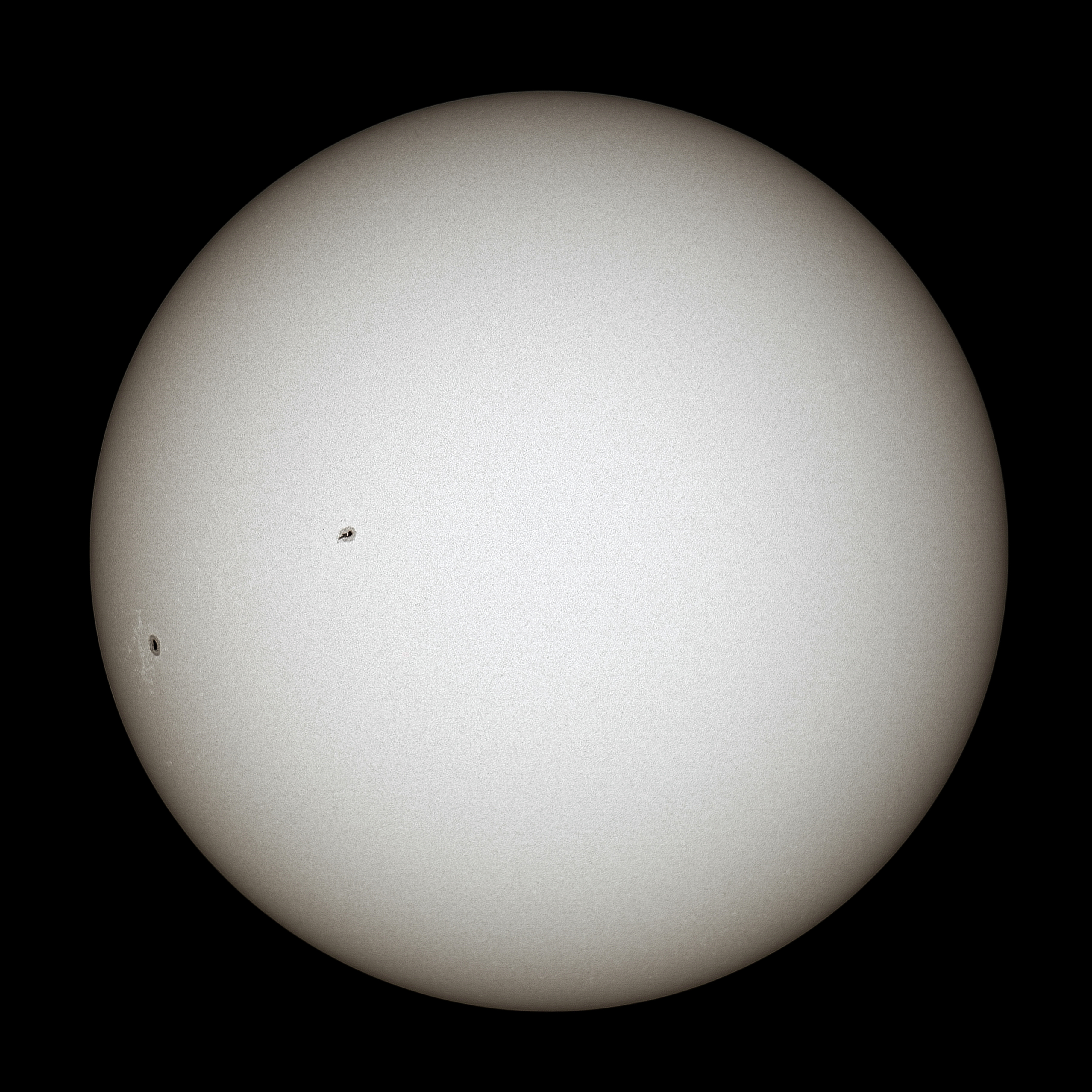
Why the Sun Burns
Nuclear Fusion
Start with two protons approaching each other.
The strong force acts only at nuclear distances, \(r\sim (1-2)~\mathrm{fm}\).
In natural units the Coulomb repulsion energy is \[ U_C(r) = \frac{\alpha}{r}. \]
Numerically, when \(r\) is quoted in fm,
\[ U_C(r) \simeq 1.44~\mathrm{MeV}\left(\frac{1~\mathrm{fm}}{r}\right). \]
Classical Barrier
- At the solar center:
\[ T_c \sim 1.5\times 10^7~\mathrm{K}, \qquad kT_c \sim 1.3\,~\mathrm{keV}. \]
The thermal energy scale is tiny: \[ k_BT_c \approx 1.3~\mathrm{keV} \ll U_C(1~\mathrm{fm}) \approx 1.44~\mathrm{MeV}. \]
Even the mean kinetic energy, \((3/2)k_BT_c\approx 1.9~\mathrm{keV}\), is far below the barrier.
Maxwell Tail
- A purely classical proton must come from the extreme Maxwell tail: \[ \exp\!\left[-\frac{E_C}{k_BT_c}\right] = \exp\!\left[-\frac{1.44~\mathrm{MeV}}{1.29~\mathrm{keV}}\right] \approx \exp(-1110) \approx 10^{-484}. \]
Classical Failure
- With deliberately generous core numbers, the geometric collision rate is enormous:
\[ \dot N_{\rm geom}\sim 4\times10^{64}\ \mathrm{s^{-1}}. \]
- The classical over-the-barrier penalty is the Maxwell tail:
\[ \dot N_{\rm class} \sim \dot N_{\rm geom}\,10^{-484} \sim 6\times10^{-420}\ \mathrm{s^{-1}}. \]
- Even assigning \(30~\mathrm{MeV}\) to every successful encounter gives
\[ P_{\rm class}\sim3\times10^{-431}\ \mathrm{W}. \]
Classical Failure
The observed solar photon luminosity is \[ L_\odot^{\rm obs} \simeq 3.83\times10^{26}~\mathrm{W}. \]
Thus \[ \frac{P_{\rm class}}{L_\odot^{\rm obs}} \sim 8\times10^{-458}. \]
Classical burning gives no Sun.
The Sun shines because fusion is a quantum tunneling problem.
The Net Reaction
- Hydrogen burning in the present Sun is summarized by
\[ 4\,{}^1\mathrm{H} \to {}^4\mathrm{He} + 2e^+ + 2\nu_e + Q. \]
- Using atomic masses as rest energies,
\[ Q \simeq 4m_{\mathrm H}-m_{{}^4\mathrm{He}} \simeq 26.73~\mathrm{MeV}. \]
- Neutrinos carry away part of this energy and leave the Sun.
Why the Sun Is Stable
- The first pp reaction is weak and very slow:
\[ p+p\to d+e^+ + \nu_e. \]
That slowness is not a defect. It sets the long main-sequence lifetime of the Sun.
Later steps are mostly strong or electromagnetic and are much faster.
The Sun is a thermostat: if the core heats up, fusion increases, pressure rises, the core expands, and it cools.
By the way, if there is no neutrino:
- No Sun.
- No Life.
Tunneling and Thermal Averaging
Coulomb Barrier
- For two nuclei with charges \(Z_a e\) and \(Z_b e\),
\[ U(r)=\frac{Z_aZ_b\alpha}{r}. \]
Classically, a particle with energy \(E<U(r)\) cannot enter the nuclear region.
Quantum mechanically, the wave function continues under the barrier and is exponentially suppressed.
WKB Probability
For the relative coordinate of two nuclei, use the one-dimensional radial WKB estimate.
In the forbidden region, \(U(r)>E\), define
\[ \kappa(r) = \sqrt{2\mu\,[U(r)-E]} . \]
- The wave amplitude decreases as
\[ \psi(r)\propto \exp\!\left[-\int \kappa(r)\,dr\right]. \]
WKB Probability
- Therefore the probability contains the square of this exponential:
\[ P(E) \sim \exp\!\left[ -2 \int_{r_N}^{r_C} \sqrt{2\mu\,[U(r)-E]}\,dr \right]. \]
- Here \(\mu\) is the reduced mass, \(r_N\) is a nuclear radius, and \(r_C\) is the outer turning point.
Gamow Factor
- For \(r_N\ll r_C\), the WKB integral gives the Gamow factor:
\[ P(E)\simeq \exp[-2\pi\eta(E)]. \]
- Indeed,
\[ 2I \simeq 2 \sqrt{2\mu E}\,r_C\,\frac{\pi}{2} = 2\pi\eta(E). \]
- For nonrelativistic charged particles, \(v=\sqrt{2E/\mu}\) and
\[ 2\pi\eta(E) = \frac{2\pi Z_aZ_b\alpha}{v} = \sqrt{\frac{E_G}{E}}, \qquad E_G = 2\mu(\pi\alpha Z_aZ_b)^2. \]
Thermal Averaging
- Thermal averaging:
\[ \langle\sigma v\rangle = \left(\frac{8}{\pi\mu}\right)^{1/2} \frac{1}{(kT)^{3/2}} \int_0^\infty \sigma(E)\,E\,e^{-E/kT}\,dE . \]
- For charged particles,
\[ \sigma(E)= \frac{S(E)}{E} \exp\!\left[-\sqrt{\frac{E_G}{E}}\right]. \]
Thermal Averaging
- This leads to the Gamow peak and the Gamow window:
\[ \langle\sigma v\rangle \propto S(E)\exp\!\left[-\frac{E}{kT}-\sqrt{\frac{E_G}{E}}\right]. \]
Gamow Window Applet
Uses $kT=1.30~\mathrm{keV}$ and
$E_G=978\,\mu(Z_1Z_2)^2~\mathrm{keV}$, with $\mu$ in atomic mass units.
The ${}^7\mathrm{Be}+p$ peak is near $18~\mathrm{keV}$.
Solar Neutrino Sources
pp Chain
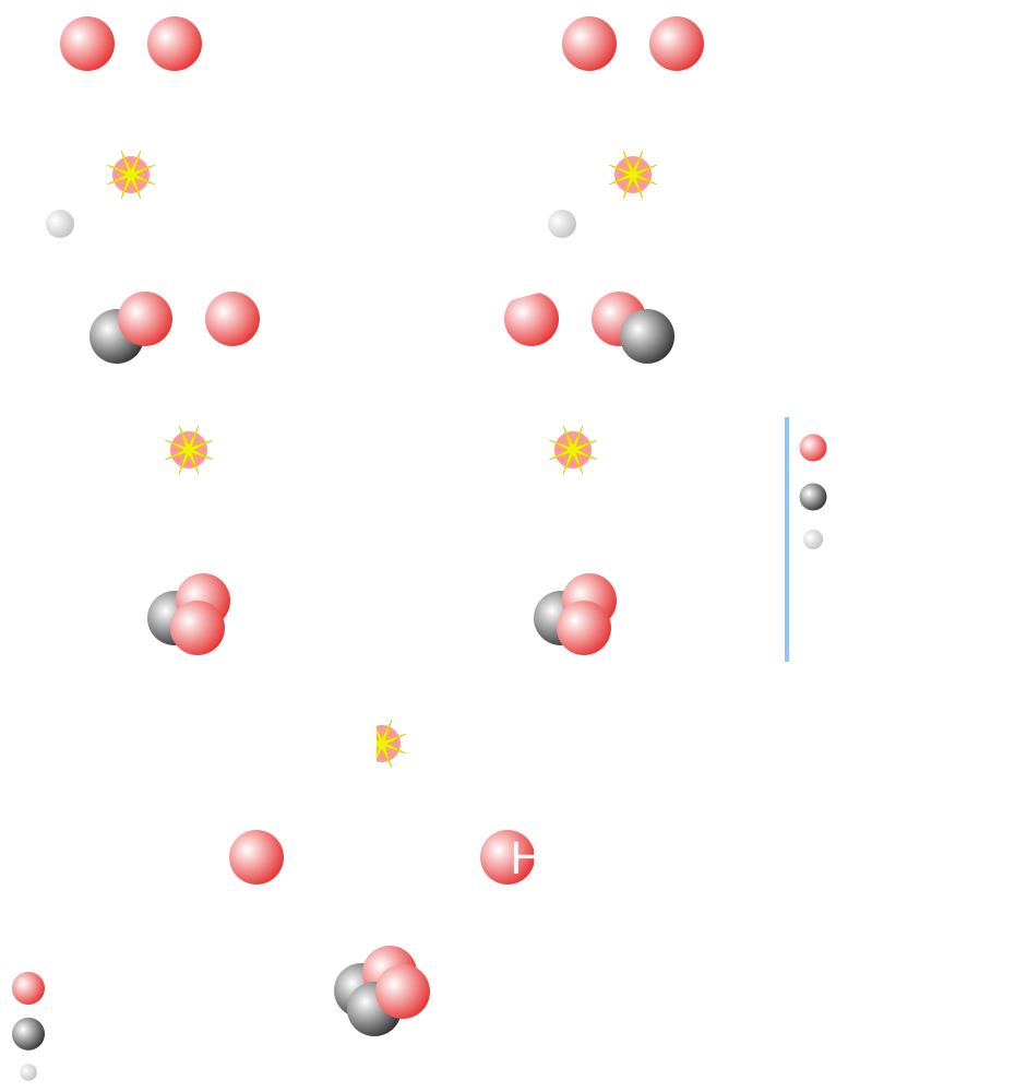
- In the present Sun, the pp chain is the main hydrogen-burning cycle and the dominant source of solar luminosity.
CNO Cycle
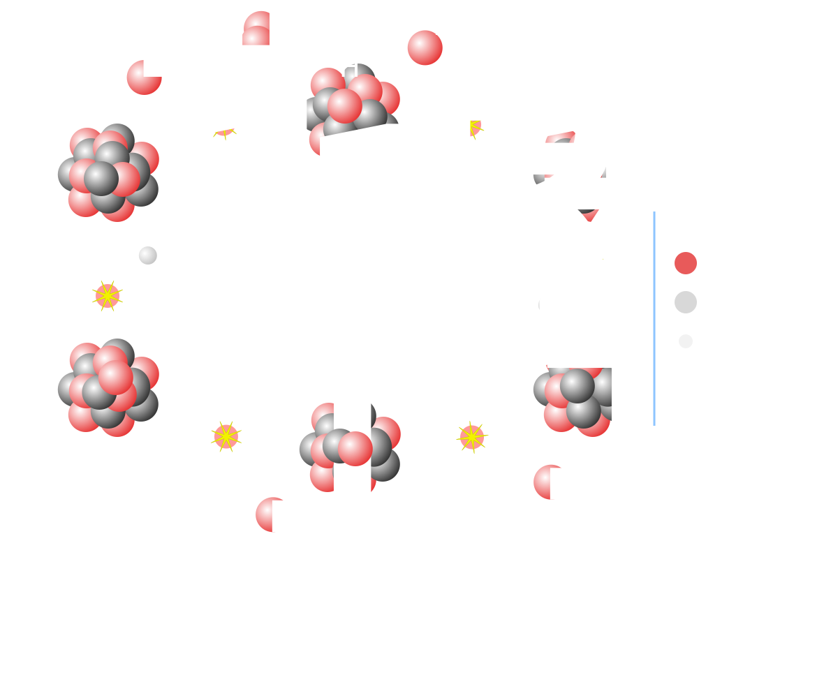
CNO catalytic loop and the smaller NO side branch.
Why CNO Matters
For the present Sun, the pp chain dominates the luminosity.
CNO neutrinos are still important because they probe:
- the metal abundance in the solar core;
- the temperature dependence of nuclear burning;
- the solar-composition problem in standard solar models.
CNO neutrinos are a composition probe, not just another low-rate component.
Flux Hierarchy
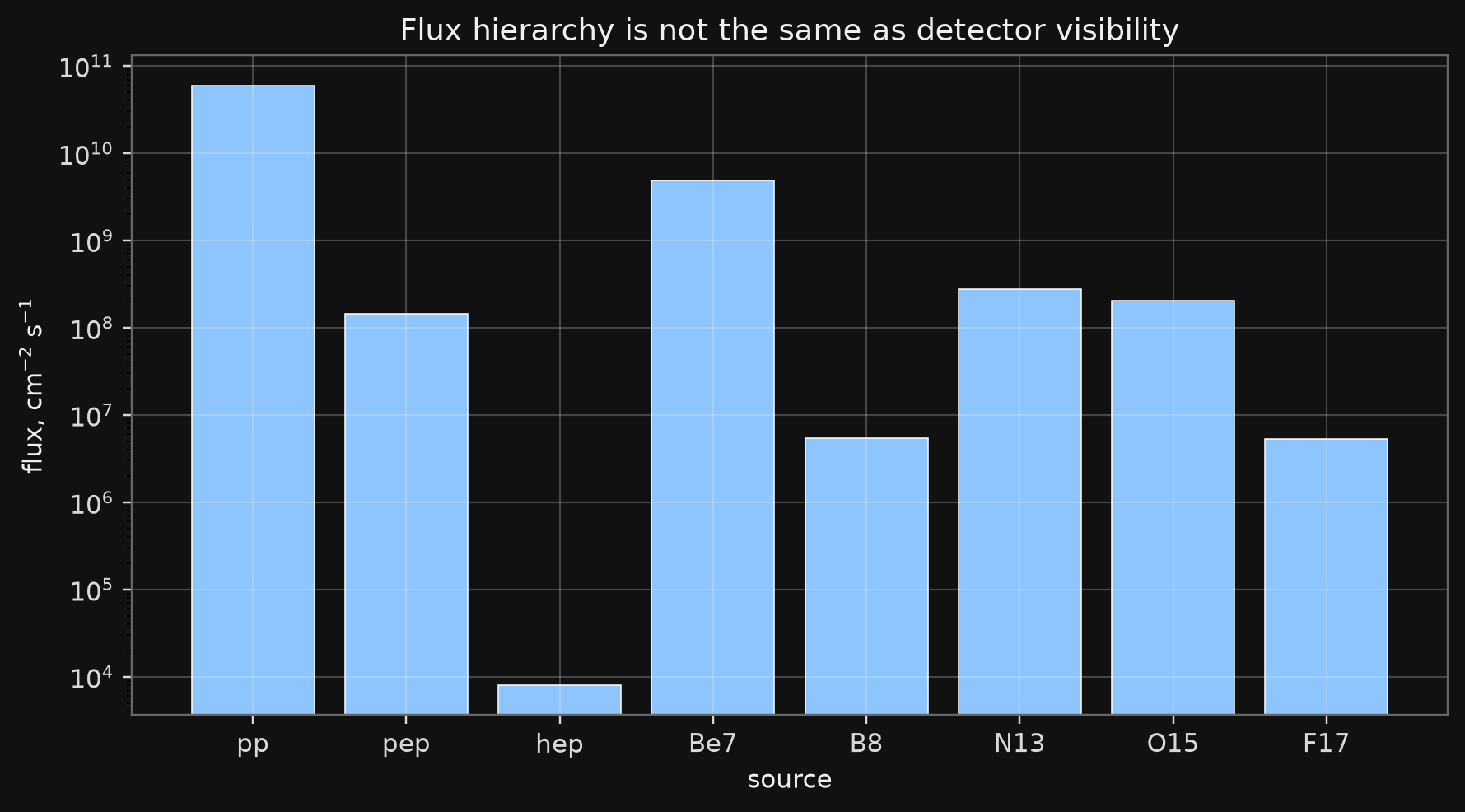
Reference numbers in the project are pedagogical values. They must be replaced by a selected SSM table for publication-level work.
Solar Neutrino Spectrum
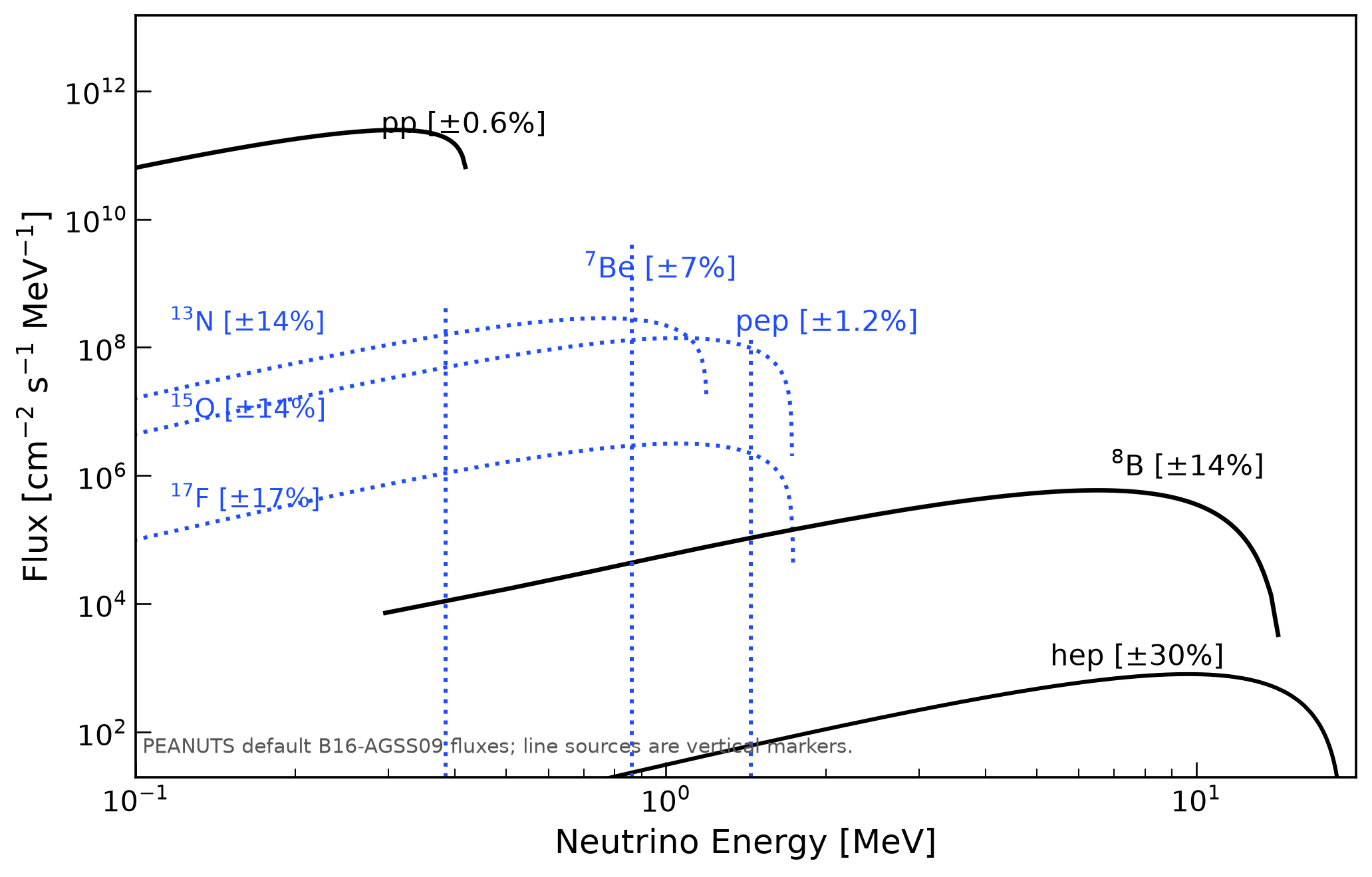
The masterclass uses generated tables. This plot is built from fluxes and normalized spectral shapes.
Radial Production
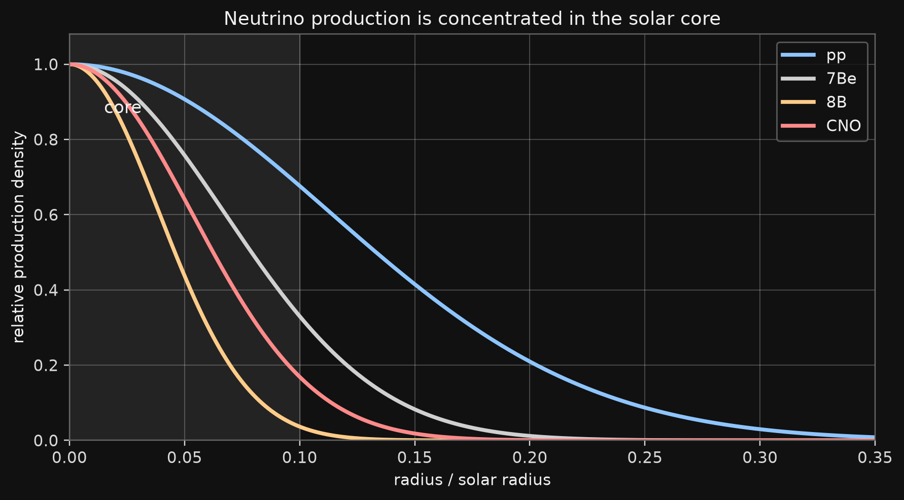
High-temperature branches are more centrally concentrated. This matters because matter effects depend on the production density.
Important Warning
The flux hierarchy is not the detector hierarchy.
The detected spectrum depends on
\[ \frac{d\Phi_i}{dE}\,P_{ee}(E)\,\sigma(E)\,\epsilon(E). \]
A huge low-energy flux can be invisible for a detector with a high threshold.
Flavor Conversion
Lepton Mixing
- Flavour states are not mass states.
\[ \begin{pmatrix} |\nu_e\rangle\\ |\nu_\mu\rangle \end{pmatrix} = \begin{pmatrix} \cos\theta & \sin\theta\\ -\sin\theta & \cos\theta \end{pmatrix} \begin{pmatrix} |\nu_1\rangle\\ |\nu_2\rangle \end{pmatrix}. \]
- Equivalently,
\[ |\nu_e\rangle=\cos\theta\,|\nu_1\rangle+\sin\theta\,|\nu_2\rangle, \qquad |\nu_\mu\rangle=-\sin\theta\,|\nu_1\rangle+\cos\theta\,|\nu_2\rangle. \]
- The angle \(\theta\) measures how different the weak-interaction basis is from the propagation basis.
Probability
Phase
\[ E_i\simeq p+\frac{m_i^2}{2E}, \qquad \Delta\phi = \frac{\Delta m^2 L}{2E}. \]
\[ \frac{\Delta m^2L}{4E} = 1.267\, \frac{\Delta m^2[\mathrm{eV}^2]\,L[\mathrm{km}]} {E[\mathrm{GeV}]}. \]
Two-flavour probabilities
\[ P_{ee} = 1-\sin^2 2\theta\, \sin^2\!\left(\frac{\Delta m^2L}{4E}\right), \]
\[ P_{e\mu} = \sin^2 2\theta\, \sin^2\!\left(\frac{\Delta m^2L}{4E}\right). \]
Why Matter Matters
Only \(\nu_e\) has the extra charged-current coherent forward scattering on electrons. This is the origin of the flavour-dependent matter potential.
Matter Potential
Forward scattering
\[ \nu_e+e^-\to\nu_e+e^- . \]
Effective interaction
\[ \mathcal{H}_{\rm CC}^{\rm eff} = \frac{G_F}{\sqrt2} \left[\bar\nu_e\gamma_\mu(1-\gamma_5)\nu_e\right] \left[\bar e\gamma^\mu(1-\gamma_5)e\right]. \]
Effective potential
\[ V_e(x) = \frac{\langle\mathrm{matter}|\mathcal{H}_{\rm CC}^{\rm eff}|\mathrm{matter}\rangle}{\langle\mathrm{matter}|\mathrm{matter}\rangle} \]
Matter Potential
Wolfenstein potential
\[ V_e(x)=\sqrt{2}\,G_F\,n_e(x). \]
Add it to the Hamiltonian
\[ H_f(x) = H_{\rm vac} + \begin{pmatrix} V_e(x) & 0\\ 0 & 0 \end{pmatrix}. \]
Neutral-current terms common to active flavours add only an irrelevant identity term.
For antineutrinos, \(V_e\to -V_e\).
Schroedinger Equation
- In the flavour basis,
\[ i\frac{d}{dx} \begin{pmatrix} \nu_e\\ \nu_x \end{pmatrix} = H_f(x) \begin{pmatrix} \nu_e\\ \nu_x \end{pmatrix}. \]
- After subtracting an irrelevant trace,
\[ H_f(x) = \frac{\Delta m^2}{4E} \begin{pmatrix} -\cos2\theta & \sin2\theta\\ \sin2\theta & \cos2\theta \end{pmatrix} + \begin{pmatrix} V_e(x) & 0\\ 0 & 0 \end{pmatrix}. \]
- For constant density, \(H_f\) is a constant \(2\times2\) matrix.
Diagonalization
- Define matter eigenstates by a rotation:
\[ \nu_f=U(\theta_m)\nu_m, \qquad U(\theta_m)= \begin{pmatrix} \cos\theta_m & \sin\theta_m\\ -\sin\theta_m & \cos\theta_m \end{pmatrix}. \]
- Choose \(\theta_m\) so that
\[ U^\dagger(\theta_m)H_fU(\theta_m) = \begin{pmatrix} \lambda_- & 0\\ 0 & \lambda_+ \end{pmatrix}. \]
Eigenvalues
- The required angle is
\[ \tan2\theta_m = \frac{\Delta m^2\sin2\theta} {\Delta m^2\cos2\theta-2EV_e}. \]
- The effective mass splitting is
\[ \Delta m_m^2 = \Delta m^2 \sqrt{ \left(\cos2\theta-\frac{2EV_e}{\Delta m^2}\right)^2 + \sin^2 2\theta }. \]
- After subtracting the trace \(\lambda_\pm=\pm\frac{\Delta m_m^2}{4E}\).
Matter Eigenstates
- In matter,
\[ |\nu_e\rangle = \cos\theta_m|\nu_1^m\rangle + \sin\theta_m|\nu_2^m\rangle . \]
\[ |\nu_\mu\rangle = -\sin\theta_m|\nu_1^m\rangle + \cos\theta_m|\nu_2^m\rangle . \]
Matter Probability
- For constant density, the vacuum formula keeps its form:
\[ P_{ee}^{\rm matter} = 1-\sin^2 2\theta_m\, \sin^2\!\left( \frac{\Delta m_m^2 L}{4E} \right). \]
- The appearance probability is
\[ P_{ex}^{\rm matter}=1-P_{ee}^{\rm matter}. \]
- In the Sun the density changes, so this is a local guide, not the final solar formula.
Limits: Vacuum and High Density
- Vacuum limit:
\[ V_e\to0: \qquad \theta_m\to\theta, \qquad \Delta m_m^2\to\Delta m^2. \]
- High-density solar limit:
\[ 2EV_e\gg\Delta m^2: \qquad \theta_m\to\frac{\pi}{2}. \]
- If the evolution is adiabatic, a produced \(\nu_e\) tracks a matter eigenstate into \(\nu_2\) in vacuum:
\[ P_{ee}^{\rm high} \simeq |\langle\nu_e|\nu_2\rangle|^2 = \sin^2\theta. \]
Limits: MSW Resonance
- The matter mixing becomes maximal when
\[ 2EV_e=\Delta m^2\cos2\theta, \qquad \theta_m=\frac{\pi}{4}. \]
- Equivalently,
\[ E_{\rm res} = \frac{\Delta m^2\cos2\theta} {2\sqrt{2}G_F n_e}. \]
- At resonance the level splitting is minimal and flavour conversion can be large if the evolution is adiabatic.
Decoherence
Solar neutrinos are produced over an extended region and detected after a long baseline.
The oscillatory phases are usually averaged by source size, energy resolution, and wave-packet separation.
For solar observables one therefore uses probabilities for exiting the Sun in mass eigenstates:
\[ P_{ee} = \sum_i P(\nu_e\to\nu_i \text{ at Sun exit}) |U_{ei}|^2. \]
- This is why the masterclass uses smooth survival probabilities rather than visible vacuum fringes.
Detection and Fit
Water Cherenkov Channel
For a Super-Kamiokande-like detector the main solar channel is elastic scattering:
\[ \nu + e^- \to \nu + e^-. \]
It is directional and sensitive mainly to high-energy solar neutrinos.
\(\nu_e\) has charged-current and neutral-current contributions.
\(\nu_\mu\) and \(\nu_\tau\) have only neutral-current contributions.
Water Cherenkov Channel
- Cherenkov photons are emitted only if the recoil electron satisfies
\[ \beta_e n > 1. \]
- For water, \(n\simeq1.33\), so
\[ T_e^{\rm Ch} = m_e\left(\frac{1}{\sqrt{1-1/n^2}}-1\right) \simeq 0.26~\mathrm{MeV}. \]
- The analysis threshold is much higher, at the MeV scale, because of backgrounds and detector response.
Event Rate
- The expected count in a true recoil-energy bin is
\[ \mu_j = N_eT_{\rm live} \int_{T_j}^{T_{j+1}}dT_e \int dE_\nu\, \frac{d\Phi_{^8\mathrm{B}}}{dE_\nu} \left[ P_{ee}(E_\nu)\frac{d\sigma_e(E_\nu,T_e)}{dT_e} + \left(1-P_{ee}(E_\nu)\right) \frac{d\sigma_x(E_\nu,T_e)}{dT_e} \right] \]
where \(\frac{d\Phi_{^8\mathrm{B}}}{dE_\nu}\) is \(^8\mathrm{B}\) spectral flux at Earth, in \(\mathrm{cm^{-2}\,s^{-1}\,MeV^{-1}}\)
and for a water detector with mass \(M\), the number of target electrons reads:
\[ N_e = 10\,N_A\,\frac{M}{18~\mathrm{g}} \]
Statistical Fit Model
- For the live example, compress the event-rate integral into visible recoil-energy bins:
\[ \mu_j(\sin^2\theta_{12},\Delta m^2_{21}) = \mathcal N \int_{T_j}^{T_{j+1}}dT_e \int dE_\nu\, \frac{d\Phi_{^8\mathrm{B}}}{dE_\nu} \left[ P_{ee}(E_\nu)\frac{d\sigma_e}{dT_e} + \left(1-P_{ee}(E_\nu)\right) \frac{d\sigma_x}{dT_e} \right]. \]
- The normalization \(\mathcal N=N_eT_{\rm live}\) is fixed; only \(\sin^2\theta_{12}\) and \(\Delta m^2_{21}\) are fitted.
Statistical Fit Model
- For the lecture-level demonstration, use the adiabatic two-flavour solar probability:
\[ P_{ee}(E) = \frac{1}{2} + \frac{1}{2}\cos2\theta_{12}\cos2\theta_m(E), \qquad \cos2\theta_m = \frac{\cos2\theta_{12}-A}{\sqrt{(\cos2\theta_{12}-A)^2+\sin^22\theta_{12}}}, \]
\[ A(E)=\frac{2EV_e}{\Delta m^2_{21}}, \qquad V_e=\sqrt2\,G_Fn_e. \]
- In the interactive, \(n_e\) is fixed to a representative \(^8\mathrm{B}\) production density. The \(\Delta m^2_{21}\) sensitivity comes from the energy-dependent MSW transition.
Likelihood and Profiles
- Pseudo-data are generated bin by bin:
\[ n_j\sim\mathrm{Pois}\left(\mu_j^{\rm true}\right). \]
- For each trial point,
\[ \ell(\sin^2\theta_{12},\Delta m^2_{21}) = \sum_j \left[ n_j\ln\mu_j-\mu_j \right] +\mathrm{const}. \]
- Plot the likelihood-ratio statistic
\[ q(\sin^2\theta_{12},\Delta m^2_{21}) = -2\left(\ell-\ell_{\max}\right). \]
Likelihood and Profiles
- Two-parameter contours use \(q=2.30\) and \(q=6.18\) as the usual \(1\sigma\) and \(2\sigma\) guides. One-dimensional errors come from profiles:
\[ q_{\rm p}(\sin^2\theta_{12}) = \min_{\Delta m^2_{21}}q, \qquad q_{\rm p}(\Delta m^2_{21}) = \min_{\sin^2\theta_{12}}q. \]
Interactive Fit: Solar Parameters
The live plot uses the same ingredients as the event-rate formula: the \(^8\mathrm{B}\) spectrum, the \(\nu e\) differential cross sections, the matter survival probability, and a Poisson likelihood.
Project Map
Master Class 1
- download the three working tables from the project page;
- read fluxes, spectra, and \(\nu e\) recoil cross sections;
- build the no-oscillation SK-like event-rate model;
- plot the \(^8\mathrm{B}\) spectrum and the recoil-electron spectrum;
- generate pseudo-data;
- fit the \(^8\mathrm{B}\) normalization with a Poisson likelihood;
- find the best fit and the one-parameter confidence interval.