Fall School on Interdisciplinary Neutrino Science · Zhuhai, 12 November 2026
Joint Institute for Nuclear Research, Dubna
Two flavors, \(\sin^2\theta=\sin^2\theta_{12}=0.3088\) (NuFIT 6.1); \(L_{\rm osc}=4\pi E/\Delta m^2\). Each event is drawn at random with \(P(\nu_e\to\nu_\mu)\).
A. Zero, as in the Standard Model
B. It depends on its mood: it is a chameleon
C. It has no mass of its own: it is a mix of \(\nu_1\), \(\nu_2\), \(\nu_3\)
A. Zero, as in the Standard Model
B. It depends on its mood: it is a chameleon
C. It has no mass of its own: it is a mix of \(\nu_1\), \(\nu_2\), \(\nu_3\)
Each of \(\nu_1\), \(\nu_2\), \(\nu_3\) has its own mass. \(\nu_e\) is their mix, so it has none of its own.
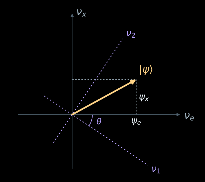
\[ \boxed{ \begin{aligned} |\nu_e\rangle&=\cos\theta\,|\nu_1\rangle+\sin\theta\,|\nu_2\rangle\\ |\nu_\mu\rangle&=-\sin\theta\,|\nu_1\rangle+\cos\theta\,|\nu_2\rangle \end{aligned}} \]
Here \(\nu_x=\nu_\mu\).
Move the detector. \(\nu_1\) and \(\nu_2\) leave the source in phase: \(\nu_e\). In antiphase the detector finds \(\nu_\mu\); in phase again, \(\nu_e\). A real geoneutrino makes about \(2\times10^{17}\) waves over \(L_{\rm osc}\approx100\) km.
Natural units
\(\hbar=c=1\)
\(E,\ p,\ m\) in eV
\(L,\ t\) in eV\(^{-1}\)
\(\hbar c=1.973\times10^{-7}\) eV m
\(\hbar=6.582\times10^{-16}\) eV s
CODATA 2022
\[ \boxed{ P(\nu_e\to\nu_\mu)=\sin^2 2\theta\;\sin^2\!\left(\frac{\Delta m^2L}{4E}\right) =\sin^2 2\theta\;\sin^2\!\left(1.267\,\frac{\Delta m^2[\mathrm{eV^2}]\;L[\mathrm{km}]}{E[\mathrm{GeV}]}\right)}, \qquad P(\nu_e\to\nu_e)=1-P(\nu_e\to\nu_\mu). \]
\[ L_{\rm osc}=\frac{4\pi E}{\Delta m^2}=2.48\ \mathrm{km}\;\frac{E[\mathrm{GeV}]}{\Delta m^2[\mathrm{eV^2}]}. \]
The first maximum of the transition is at \(L=L_{\rm osc}/2\).
Let \(\varphi_i\) be the phase that mass component \(i\) accumulates between the source and the detector:
\[ |\nu_e;L\rangle=\cos\theta\,e^{-i\varphi_1}|\nu_1\rangle+\sin\theta\,e^{-i\varphi_2}|\nu_2\rangle . \]
A single mass state would carry only an overall phase, invisible in any probability. Here there are two waves: after the common factor is taken out, the difference \(\Delta\varphi=\varphi_2-\varphi_1\) remains.
The detector looks for \(|\nu_\mu\rangle=-\sin\theta\,|\nu_1\rangle+\cos\theta\,|\nu_2\rangle\). The mass states are orthonormal, \(\langle\nu_i|\nu_j\rangle=\delta_{ij}\), and two terms survive:
\[ \mathcal A_{e\to\mu}=\langle\nu_\mu|\nu_e;L\rangle =\sin\theta\cos\theta\left(e^{-i\varphi_2}-e^{-i\varphi_1}\right). \]
At \(L=0\) the phases are equal and the two terms cancel: the source prepared a pure \(\nu_e\).
\[ \left|e^{-i\varphi_2}-e^{-i\varphi_1}\right|^2=4\sin^2\frac{\Delta\varphi}{2}, \qquad 4\sin^2\theta\cos^2\theta=\sin^22\theta, \qquad P(\nu_e\to\nu_\mu)=\sin^22\theta\,\sin^2\frac{\Delta\varphi}{2}. \]
For a plane wave \(\varphi_i=E_it-p_iL\). With \(t\simeq L\) (\(\hbar=c=1\)) and \(E_i^2-p_i^2=m_i^2\):
\[ \varphi_i\simeq(E_i-p_i)L=\frac{m_i^2L}{E_i+p_i}\simeq\frac{m_i^2L}{2E}, \qquad \Delta\varphi\simeq\frac{\Delta m^2L}{2E}. \]

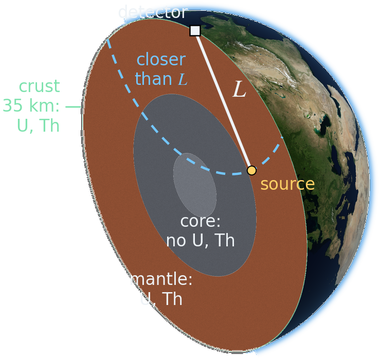
One source at distance \(L\): \(P_{ee}(L)\). All sources of the Earth closer than \(L\): \(\bar P_{ee}(L)=\int_0^L w(x)\,P_{ee}(x)\,dx\Big/\!\int_0^L w(x)\,dx\).
A volume \(dV\) emitting \(n\) antineutrinos per cm³ per s gives the flux \(n\,dV/4\pi x^2\); around the detector \(dV=x^2dx\,d\Omega\), so \(d\Phi=\frac{n}{4\pi}\,dx\,d\Omega\). Only the solid angle inside a shell \(a<r<b\) is left; \(\beta\) is the angle from the vertical, \(r^2=R^2+x^2-2Rx\cos\beta\):
\[ \frac{d\Phi}{dx}=\frac{n}{2}\,\bigl[\cos\beta(a)-\cos\beta(b)\bigr], \qquad \cos\beta(r)=\frac{R^2+x^2-r^2}{2Rx}\ \ \text{clipped to}\ [-1,1]. \]
The detector does not know where a neutrino came from; it counts all of them:
\[ S(L)=\sum_{\rm shells}\int_0^L \frac{d\Phi}{dx}\,P_{ee}(x)\,dx, \qquad w(x)=\frac{1}{S_0}\sum_{\rm shells}\frac{d\Phi}{dx}, \qquad S_0:\ \text{the whole Earth without oscillations.} \]
Continental crust 35 km (Rudnick & Gao 2003); mantle: bulk silicate Earth (McDonough & Sun 1995) minus the crust; TNU after Fiorentini et al. 2007. Spectrum: U and Th chains (S. Enomoto) times the IBD cross section (Vogel & Beacom 1999), U : Th = 30.3 : 9.0 TNU. Oscillations: NuFIT 6.1, normal ordering. Earth picture: radii to scale, interior colors schematic; surface: NASA Blue Marble.

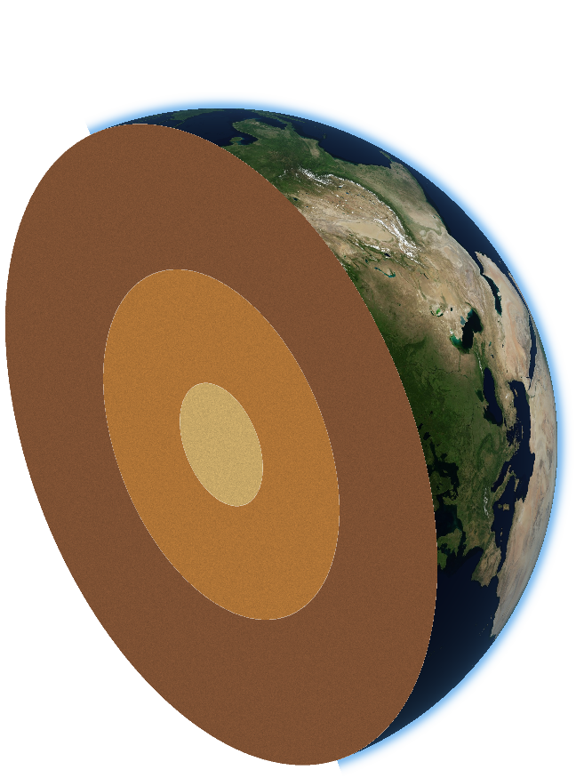
A \(\nu_\mu\) born in the atmosphere at height \(h\approx15\) km; the zenith angle fixes the path: \(L=15\) km from above, \(437\) km from the horizon, \(12\,757\) km from below.
The path from the birth point at height \(h\) to a detector on the surface, \(R=6371\) km:
\[ L(\theta_z)=\sqrt{(R+h)^2-R^2\sin^2\theta_z}-R\cos\theta_z , \qquad h\approx15\ \text{km}. \]
Three flavors in vacuum, one energy and one direction:
\[ P(\nu_\mu\to\nu_\beta)=\Bigl|\sum_{i=1}^{3}U_{\beta i}\,U^*_{\mu i}\,e^{-i m_i^2L/2E}\Bigr|^2 . \]
\(h\approx15\) km: the most probable production height of vertical neutrinos from pion decay (Gaisser & Stanev, Phys. Rev. D 57, 1977 (1998)). NuFIT 6.1 best fit (IC24 + SK-atm), normal ordering: \(\sin^2\theta_{12}=0.3088\), \(\sin^2\theta_{13}=0.02248\), \(\sin^2\theta_{23}=0.470\), \(\delta=212^\circ\), \(\Delta m^2_{21}=7.537\times10^{-5}\) eV², \(\Delta m^2_{31}=2.511\times10^{-3}\) eV². Earth picture: radii to scale (PREM), interior colors schematic; surface: NASA Blue Marble.

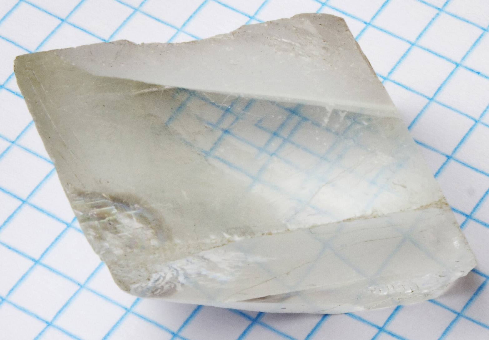
Calcite on graph paper: every line is seen twice. Photo: APN MJM, Wikimedia Commons, CC BY-SA 3.0.
In. The polarizer passes light polarized along \(H\).
Crystal, thickness \(L\), axes at the angle \(\theta\) to \(H\): two waves, \(\cos\theta\) along the fast axis, \(\sin\theta\) along the slow one.
Out. The slow wave lags by \(\Delta\varphi=2\pi\,(n_o-n_e)\,L/\lambda\): the polarization is elliptical.
Filter \(V\). The detector sees \(I_V/I_0=\sin^22\theta\,\sin^2(\Delta\varphi/2)\).
Calcite at 589 nm: \(n_o=1.658\), \(n_e=1.486\) (G. Ghosh, Opt. Commun. 163, 95 (1999)); a full-wave plate is \(\lambda/(n_o-n_e)=3.42\ \mu\)m thick. The drawing is schematic: wavelength and thickness not to scale.
In the mass basis the vacuum is diagonal: one refractive index per mass state,
\[ n=\begin{pmatrix}n_1&0&0\\0&n_2&0\\0&0&n_3\end{pmatrix}, \qquad n_i\simeq1-\frac{m_i^2}{2E^2}, \qquad E\,(n_i-n_j)\,L=\frac{\Delta m^2_{ji}\,L}{2E}. \]
| Light in calcite | Neutrinos in vacuum |
|---|---|
| two axes, \(o\) and \(e\) | three axes, \(\nu_1,\nu_2,\nu_3\) |
| angle \(\theta\) of the axes to \(H\) | mixing angles \(\theta_{12},\theta_{13},\theta_{23}\) |
| polarizer \(H\), analyzer \(V\) | \(\nu_e\) at the source, \(\nu_\mu\) at the detector |
| \(\Delta\varphi=2\pi\,(n_o-n_e)\,L/\lambda\) | \(\Delta\varphi_{ji}=\Delta m^2_{ji}\,L/2E\) |
Three neutrinos, three axes: even empty space is a crystal for them.
| \(\Delta n\) | a full turn of the phase | ||
|---|---|---|---|
| light, 589 nm | calcite: \(n_o-n_e\) | \(0.17\) | \(3.4\ \mu\mathrm{m}\) |
| \(\nu\), 10 MeV | vacuum: \(n_1-n_2\) | \(3.8\times10^{-19}\) | \(329\ \mathrm{km}\) |
| \(\nu\), 10 MeV | solar center: \(n_{\nu_\mu}-n_{\nu_e}\) | \(7.9\times10^{-19}\) | \(158\ \mathrm{km}\) |
\(5\times10^{17}\) times weaker than calcite. The flavor still turns: the paths are hundreds of kilometers.
\(\Delta n=\Delta m^2_{21}/2E^2\) and \(V/E\) with \(V=\sqrt2\,G_Fn_e\), \(n_e/N_A=102.9\ \mathrm{cm^{-3}}\) at the solar center (BS05(OP)); a full turn: \(E\,\Delta n\,L=2\pi\).
A. Above \(c\)
B. Below \(c\), as for light in glass
C. Whatever the solar weather allows today
A. Above \(c\)
B. Below \(c\), as for light in glass
C. Whatever the solar weather allows today
\(n_{\nu_e}-1=-V/E<0\): the phase runs faster than light. The group velocity, which carries the signal, stays below \(c\). Einstein is safe.
\[ \boxed{\,n_{\nu_e}-1=-\frac{V}{E}<0\,}, \qquad V=\sqrt2\,G_F\,n_e . \]
\[ n-1=-\frac{V}{E}\begin{pmatrix}1&0\\0&0\end{pmatrix}: \ \text{the axes } \nu_e,\nu_\mu \text{ stay.} \]
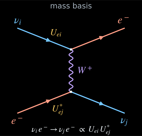
The same scattering, written for \(\nu_1,\nu_2\) (\(U_{e1}=\cos\theta\), \(U_{e2}=\sin\theta\)):
\[ n-1=-\frac{V}{E}\begin{pmatrix}\cos^2\theta&\sin\theta\cos\theta\\\sin\theta\cos\theta&\sin^2\theta\end{pmatrix}. \]
The crystal turns its axes, \(\nu_{1,2}\to\nu_{1m,2m}\), and its indices change, \(n_{1,2}\to n_{1m,2m}\).
A plane wave \(e^{ikz}\) crosses a slab \(dz\) with \(N\) scatterers per volume, each scattering \(f(\theta)\,e^{ikr}/r\). The first Fresnel zones add up to
\[ e^{ikz}\Bigl[1+\frac{2\pi i}{k}\,N f(0)\,dz\Bigr]=e^{inkz} \quad\Rightarrow\quad n-1=\frac{2\pi N f(0)}{k^2}. \]
Only the forward amplitude \(f(0)\) enters.
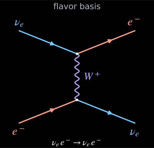
\(W\) exchange at \(q^2\ll M_W^2\), after the Fierz rearrangement (coefficient \(+1\) for anticommuting fields):
\[ \mathcal L=-\frac{G_F}{\sqrt2}\,[\bar\nu_e\gamma^\mu(1-\gamma_5)\nu_e]\,[\bar e\gamma_\mu(1-\gamma_5)e]. \]
Forward, left-handed \(\nu_e\), unpolarized \(e^-\) at rest: \(\bar u_\nu\gamma^\mu(1-\gamma_5)u_\nu=4p^\mu\), \(\langle\bar u_e\gamma_\mu(1-\gamma_5)u_e\rangle=2k_\mu\):
\[ \mathcal M_{\rm fwd}=-4\sqrt2\,G_F\,E\,m_e, \qquad f(0)=\frac{\mathcal M_{\rm fwd}}{8\pi m_e}=-\frac{G_F E}{\sqrt2\,\pi}<0 . \]
Born: \(f=-\dfrac{E}{2\pi}\displaystyle\int U\,d^3r\), so \(U=\sqrt2\,G_F\,\delta^3(\mathbf r)\). A vector exchange between like charges: repulsion; \(\bar\nu_e\): \(V\to-V\).
\[ V=N_e\!\int U\,d^3r=-\frac{2\pi N_e f(0)}{E}=\sqrt2\,G_F N_e>0, \qquad n-1=-\frac{\sqrt2\,G_F N_e\,E}{p^2}\simeq-\frac{V}{E}<0 . \]
The role of \(\omega_0\). Light on an oscillator: \(f(0)=r_e\,\omega^2/(\omega_0^2-\omega^2)\); a free electron, \(\omega_0=0\): \(f(0)=-r_e\), \(n<1\) (X-rays). Here the pole is the \(W\): for \(\nu_e e^-\) it sits in the \(u\) channel and is never reached, \(n<1\) at all energies; for \(\bar\nu_e e^-\) it is in the \(s\) channel, at \(E=M_W^2/2m_e\approx6.3\) PeV (Glashow): below it \(n>1\).
R. D. Peccei, hep-ph/9906509, Eqs. (91)–(92); E. Kh. Akhmedov, hep-ph/0001264, Eqs. (84)–(88); L. Wolfenstein, Phys. Rev. D 17, 2369 (1978). \(Z\) exchange is common to all flavors and drops out.
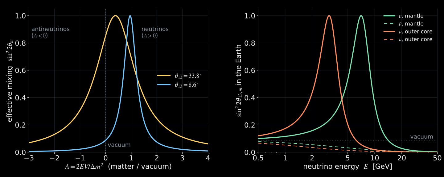
\[ \boxed{A=\frac{V}{\Delta m^2/2E}=\frac{2EV}{\Delta m^2}}, \qquad V=\sqrt2\,G_Fn_e=7.63\times10^{-14}\ \mathrm{eV}\cdot\frac{Y_e\rho}{\mathrm{g\,cm^{-3}}}, \qquad \bar\nu:\ A<0 . \]
| \(E\) | \(\Delta m^2\) | \(Y_e\rho\), g/cm³ | \(A\) | |
|---|---|---|---|---|
| solar center, \(\nu_e\) | 10 MeV | \(\Delta m^2_{21}\) | 103 | \(2.08\) |
| mantle, geo-\(\bar\nu_e\) | 3 MeV | \(\Delta m^2_{21}\) | 2.2 | \(-0.013\) |
| mantle, atmospheric \(\nu\) | 6 GeV | \(\Delta m^2_{31}\) | 2.2 | \(0.80\) |
The Sun: matter wins. Geoneutrinos: vacuum wins, 75 times. GeV neutrinos in the Earth: a draw.
After a length \(L\) each state collects the phase \(E\,(1-n)\,L\). In the basis \(\nu_1,\nu_2\):
\[ E\,(1-n)\,L=\underbrace{\varphi_0\,\mathbf{1}}_{\text{same for all}} +\underbrace{\frac{L}{2E}\begin{pmatrix}0&0\\0&\Delta m^2\end{pmatrix}}_{\text{vacuum}} +\underbrace{V L\begin{pmatrix}\cos^2\theta&\sin\theta\cos\theta\\\sin\theta\cos\theta&\sin^2\theta\end{pmatrix}}_{\text{matter}} \]
\(\varphi_0\) is not seen. Take out \(\dfrac{\Delta m^2L}{2E}=2\pi\dfrac{L}{L_{\rm osc}}\):
\[ E\,(1-n)\,L=\varphi_0\,\mathbf{1}+2\pi\,\frac{L}{L_{\rm osc}}\, \boxed{\begin{pmatrix}0&0\\0&1\end{pmatrix}+A\begin{pmatrix}\cos^2\theta&\sin\theta\cos\theta\\\sin\theta\cos\theta&\sin^2\theta\end{pmatrix}}, \qquad A=\frac{2EV}{\Delta m^2}. \]
The box is a matrix of numbers: the crystal.
In its own axes \(\nu_{1m},\nu_{2m}\) the crystal is diagonal: each axis keeps its own phase, nothing mixes.
\[ \psi_{km}(L)=e^{-2\pi i\,\lambda_k L/L_{\rm osc}}\,\psi_{km}(0), \qquad \lambda_{1,2}=\tfrac12\bigl(1+A\mp R\bigr), \qquad R=\sqrt{(\cos2\theta-A)^2+\sin^22\theta}. \]
\[ \nu_e=\cos\theta_m\,\nu_{1m}+\sin\theta_m\,\nu_{2m}, \qquad \sin2\theta_m=\frac{\sin2\theta}{R}, \qquad \cos2\theta_m=\frac{\cos2\theta-A}{R}. \]
The phase between the axes grows as \(2\pi R\,L/L_{\rm osc}\). In vacuum, \(A=0\): \(R=1\), \(\theta_m=\theta\).
\[ \boxed{P(\nu_e\to\nu_\mu)=\sin^22\theta_m\,\sin^2\!\left(\frac{\Delta m^2_m\,L}{4E}\right)} \]
\[ \sin^22\theta_m=\frac{\sin^22\theta}{(\cos2\theta-A)^2+\sin^22\theta}, \qquad \Delta m^2_m=\Delta m^2\sqrt{(\cos2\theta-A)^2+\sin^22\theta}. \]
The vacuum formula with \(\theta\to\theta_m\) and \(\Delta m^2\to\Delta m^2_m\).
A. A \(\nu_e\), of course
B. Almost only \(\nu_2\)
C. Nothing: the Sun keeps it as a souvenir
A. A \(\nu_e\), of course
B. Almost only \(\nu_2\)
C. Nothing: the Sun keeps it as a souvenir
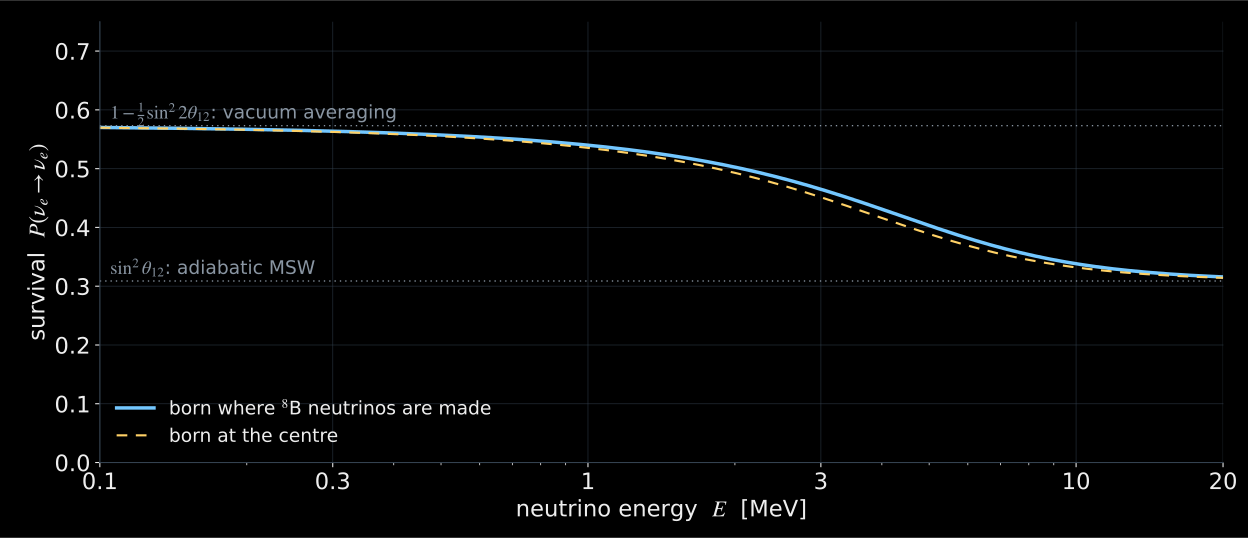
About 94 % \(\nu_2\), a mass state: it no longer oscillates on the way to the Earth. Two flavors, adiabatic; see the next slide.
Curve: three flavors, adiabatic MSW, NuFIT 6.1, BS05(OP) density where \(^8\)B neutrinos are made. Points: Borexino with high-metallicity solar fluxes, Nature 562, 505 (2018); values as quoted in arXiv:2105.13858.
Three flavors, three masses: \(\nu_\alpha=\sum_{i=1}^{3}U_{\alpha i}\,\nu_i\), \(\alpha=e,\mu,\tau\). Both sets are orthonormal bases of one space, so \(U\) is unitary:
\[ UU^\dagger=U^\dagger U=\mathbf 1:\qquad \underbrace{\sum_{i}|U_{\alpha i}|^2=1}_{\text{rows}},\qquad \underbrace{\sum_{\alpha}|U_{\alpha i}|^2=1}_{\text{columns}},\qquad \underbrace{\sum_{\alpha}U_{\alpha i}U^*_{\alpha j}=0,\ i\ne j}_{\text{orthogonal columns}} . \]
\(|U_{\alpha i}|^2\) is the share of \(\nu_i\) in \(\nu_\alpha\). Two measurements, to leading order:
\[ \text{solar }{}^8\text{B}:\ P_{ee}\simeq|U_{e2}|^2\simeq\tfrac13, \qquad \text{atmospheric}:\ 4|U_{\mu3}|^2\bigl(1-|U_{\mu3}|^2\bigr)\simeq1, \qquad |U_{e3}|^2\simeq0 . \]
Nine shares \(|U_{\alpha i}|^2\): two measurements, \(|U_{e3}|^2\simeq0\) and unitarity fix them all.
The rows correspond to the flavors of production and detection; the columns, to the mass states. We begin with the measurable fractions \(|U_{\alpha i}|^2\).
For now we leave \(|U_{e3}|^2=0\). This reveals the framework of the problem; the reactor result will be included at the end.
For high-energy solar neutrinos \(P_{ee}\simeq1/3\). In the adiabatic approximation and for \(U_{e3}=0\):
\(P_{ee}\simeq |U_{e2}|^2\simeq\frac13.\)
The Sun turns a \(\nu_e\) into \(\nu_2\): the adiabatic MSW effect (appendix, "Follow the twist").
Its normalization fills the remaining cell:
\( |U_{e1}|^2+|U_{e2}|^2+|U_{e3}|^2=1 \quad\Longrightarrow\quad |U_{e1}|^2=\frac23. \)
The first row is now equal to \((2/3,\,1/3,\,0)\).
The nearly maximal disappearance \(\nu_\mu\) shows that the muon flavor is distributed roughly equally with respect to the third mode:
\( 4|U_{\mu3}|^2(1-|U_{\mu3}|^2)\simeq1 \quad\Longrightarrow\quad |U_{\mu3}|^2\simeq\frac12. \)
Here we keep the leading atmospheric scale and for now set \(U_{e3}=0\).
The three fractions of a single mass state sum to one:
\( |U_{e3}|^2+|U_{\mu3}|^2+|U_{\tau3}|^2=1 \quad\Longrightarrow\quad |U_{\tau3}|^2=\frac12. \)
In this approximation \(\nu_3\) is equally coupled to \(\nu_\mu\) and \(\nu_\tau\).
From column 3 we already know \(|U_{\mu3}|=|U_{\tau3}|\). Its orthogonality to column 2 gives
\( U_{\mu2}^*U_{\mu3}+U_{\tau2}^*U_{\tau3}=0. \)
Therefore, \(|U_{\mu2}|^2=|U_{\tau2}|^2\). We normalize the second column:
\( \frac13+|U_{\mu2}|^2+|U_{\tau2}|^2=1. \)
\( |U_{\mu2}|^2=|U_{\tau2}|^2=\frac13. \)
We normalize the muon and tau rows:
\( |U_{\mu1}|^2=1-\frac13-\frac12=\frac16, \qquad |U_{\tau1}|^2=\frac16. \)
All rows and columns of the matrix of squares now sum to one.
Each cell on the right so far contains the probability \(|U_{\alpha i}|^2\). We take the square root:
\( |U_{\alpha i}|=\sqrt{|U_{\alpha i}|^2}, \qquad |U_{e1}|=\sqrt{\frac23},\quad |U_{\mu1}|=\sqrt{\frac16}. \)
The matrix of non-negative moduli is not yet \(U\): its columns are not orthogonal. The relative signs are missing.
Denote the columns by \(c_1,c_2,c_3\). For a real representative we choose as positive \(U_{e2},U_{\mu2},U_{\mu3},U_{\tau3}\). From the orthogonality of columns 2 and 3 it follows that
\( c_2\!\cdot c_3= U_{\mu2}U_{\mu3}+U_{\tau2}U_{\tau3}=0. \)
\( U_{\tau2}=-U_{\mu2}=-\sqrt{\frac13}. \)
The first column is so far shown in absolute value: we will find its signs from the next condition.
Choose \(U_{e1}>0\). Orthogonality with the third column gives \(U_{\mu1}=-U_{\tau1}\). With the second:
\( c_1\!\cdot c_2= \sqrt{\frac13} (U_{e1}+U_{\mu1}-U_{\tau1})=0. \)
\( U_{\mu1}=-\sqrt{\frac16},\qquad U_{\tau1}=+\sqrt{\frac16}. \)
We obtained \(U_0^{\mathsf T}U_0=I\): the column norms are equal to one, and the pairwise scalar products are zero.
The signs of this representative depend on the choice of the state phases. For \(U_{e3}=0\) the phase \(\delta_{\rm CP}\) is not observed in oscillations.
A measurement at the near and far detectors gives \(|U_{e3}|^2=\sin^2\theta_{13}\simeq0.0225\). The matrix on the right is an example \(|U|^2\), calculated from the best-fit point of NuFIT 6.1.
Appearance channels and antiparticles provide information about \(\delta_{\rm CP}\). The squared moduli alone do not determine all the complex phases \(U\).
The numbers on the right are calculated in the unitary model. For an independent test of unitarity, this condition is lifted in the data analysis.
| \(\nu_1\) | \(\nu_2\) | \(\nu_3\) | |
|---|---|---|---|
| \(e\) | \(\tfrac23\)\(\sqrt{\tfrac23}\)\(\pm\sqrt{\tfrac23}\)\(+\sqrt{\tfrac23}\)\(0.676\) | \(\tfrac13\)\(\sqrt{\tfrac13}\)\(+\sqrt{\tfrac13}\)\(+\sqrt{\tfrac13}\)\(0.302\) | \(0\)\(0\)\(0\)\(0\)\(0.022\) |
| \(\mu\) | \(\tfrac16\)\(\sqrt{\tfrac16}\)\(\pm\sqrt{\tfrac16}\)\(-\sqrt{\tfrac16}\)\(0.112\) | \(\tfrac13\)\(\sqrt{\tfrac13}\)\(+\sqrt{\tfrac13}\)\(+\sqrt{\tfrac13}\)\(0.428\) | \(\tfrac12\)\(\sqrt{\tfrac12}\)\(+\sqrt{\tfrac12}\)\(+\sqrt{\tfrac12}\)\(0.459\) |
| \(\tau\) | \(\tfrac16\)\(\sqrt{\tfrac16}\)\(\pm\sqrt{\tfrac16}\)\(+\sqrt{\tfrac16}\)\(0.212\) | \(\tfrac13\)\(\sqrt{\tfrac13}\)\(-\sqrt{\tfrac13}\)\(-\sqrt{\tfrac13}\)\(0.270\) | \(\tfrac12\)\(\sqrt{\tfrac12}\)\(+\sqrt{\tfrac12}\)\(+\sqrt{\tfrac12}\)\(0.518\) |
| NuFIT 6.1 | JUNO, 59.1 d | JUNO, 207.2 d | |
|---|---|---|---|
| \(\sin^2\theta_{12}\) | 0.3088 | \(0.3092\pm0.0087\) | \(0.3036\pm0.0064\) |
| \(\Delta m^2_{21}/10^{-5}\,\mathrm{eV^2}\) | 7.537 | \(7.50\pm0.12\) | \(7.388\pm0.078\) |
| \(\sin^2\theta_{13}\) | 0.02248 | ||
| \(\sin^2\theta_{23}\) | 0.470 | ||
| \(\Delta m^2_{31}/10^{-3}\,\mathrm{eV^2}\) | \(+2.511\) | \(+2.509^{+0.027}_{-0.025}\) | |
| \(\delta_{CP}\) | \(212^\circ\) |
Open
NuFIT 6.1, best fit, normal ordering, IC24 with SK atmospheric data (www.nu-fit.org). JUNO: arXiv:2511.14593 (59.1 days), arXiv:2609.37895 (207.2 days, normal ordering).

Quantum Field Theory for Experimentalists and Beyond
A practical course with examples, problems, and solutions: from the foundations to renormalization, anomalies and functional integrals, always tied to experiment.
At fixed energy, in the mass basis, with \(\Delta=\Delta m^2/2E\) (terms common to both states dropped):
\[ i\frac{d}{dx}\binom{\psi_1}{\psi_2}= \left[ \begin{pmatrix}0&0\\0&\Delta\end{pmatrix} +V\begin{pmatrix}\cos^2\theta&\sin\theta\cos\theta\\\sin\theta\cos\theta&\sin^2\theta\end{pmatrix} \right] \binom{\psi_1}{\psi_2}. \]
The first matrix is the vacuum, diagonal. The second is \(V\) times the projector on \(\nu_e=\cos\theta\,\nu_1+\sin\theta\,\nu_2\): \(\nu_1\) and \(\nu_2\) are no longer eigenstates. In units of \(\Delta\) this is the matrix \(\mathrm{diag}(0,1)+A\,P_e\) of the slide “Matter turns the axes”.
In units of \(\Delta\) the matrix is \(M=\begin{pmatrix}A\cos^2\theta&A\sin\theta\cos\theta\\A\sin\theta\cos\theta&1+A\sin^2\theta\end{pmatrix}\), with \(\operatorname{tr}M=1+A\) and \(\det M=A\cos^2\theta\). Then \(\det(M-\lambda)=0\) gives
\[ \lambda_{1,2}=\frac{1+A\mp\sqrt{(1+A)^2-4A\cos^2\theta}}{2}=\frac{1+A\mp R}{2}, \qquad (1+A)^2-4A\cos^2\theta=(\cos2\theta-A)^2+\sin^22\theta=R^2 . \]
The phase difference is \((\lambda_2-\lambda_1)\Delta L=R\,\Delta m^2L/2E\): hence \(\Delta m^2_m=R\,\Delta m^2\). Its smallest value, \(R=\sin2\theta\), is at \(A=\cos2\theta\): the levels would cross there; mixing keeps them apart.
Rotate to the flavor basis, \(\nu_e=\cos\theta\,\nu_1+\sin\theta\,\nu_2\):
\[ M_{\rm flavor}=\frac{1+A}{2}\,\mathbf 1+\frac12\begin{pmatrix}A-\cos2\theta&\sin2\theta\\\sin2\theta&\cos2\theta-A\end{pmatrix} =\frac{1+A}{2}\,\mathbf 1+\frac R2\begin{pmatrix}-\cos2\theta_m&\sin2\theta_m\\\sin2\theta_m&\cos2\theta_m\end{pmatrix}, \]
\[ \sin2\theta_m=\frac{\sin2\theta}{R},\qquad \cos2\theta_m=\frac{\cos2\theta-A}{R}. \]
The same form as the vacuum (\(A=0\), \(R=1\)) with \(\theta\to\theta_m\): the eigenvectors are \(\nu_{1m}=\cos\theta_m\,\nu_e-\sin\theta_m\,\nu_\mu\), \(\nu_{2m}=\sin\theta_m\,\nu_e+\cos\theta_m\,\nu_\mu\), and the vacuum derivation of \(P\) repeats with \(\theta\to\theta_m\), \(\Delta m^2\to R\,\Delta m^2\).
“Adiabatic”: the state follows the upper branch and leaves as the other flavor. “Fast”: it jumps across the gap. “Small θ”: the gap is narrow and following is harder.
P₁ + P₂ = 1 exactly, no averaging
Push one pendulum: the swing moves to the other one and back. Each normal mode keeps its own frequency; the energy transfer is their beat, \(P_{1\to2}(t)=\sin^22\theta\,\sin^2[(\omega_--\omega_+)t/2]\).