Direct Determination of the Neutrino Mass.
MAC-E Spectrometer

Introduction to Neutrino Physics

Dmitry V. Naumov

JINR

MAC-E filter

How to make the threshold almost independent of the angle?

Notation

  • \(\mathrm{src}\) — the source region (from the English source),

  • \(\mathrm A\) — the analyzing plane.

  • \(U\) — the retarding voltage; \(e>0\) — the magnitude of the electron charge.

  • The neutrino mass changes the shape of the \(\beta\) spectrum.

  • The electrostatic barrier is sensitive to the longitudinal energy of the electron.

  • In the analyzing plane

\[ \boxed{ E_{\parallel,\mathrm A} \simeq E-e|U|-E_{\perp,\mathrm A} }. \]

  • Electrons of the same energy are born at different angles and have different \(E_\perp\).

  • We need to achieve

\[ \boxed{E_{\perp,\mathrm A}\ll E} \]

  • This condition must hold for a large solid angle, and not only for electrons moving along the axis.
  • In a uniform field

\[ p_\parallel=\mathrm{const}, \qquad p_\perp=\mathrm{const}, \qquad \alpha=\mathrm{const}. \]

  • The field guides the guiding center to the detector, but does not collimate the beam.

  • For the fast cyclotron motion we introduced the action

\[ \boxed{ J=\frac{1}{2\pi}\oint P\,dQ =\frac{E_\perp}{\omega_c} =\frac{p_\perp^2}{2|q|B} }. \]

  • In a constant uniform field \(J\) is conserved exactly.

  • Is \(J\) conserved in a nonuniform field?

    • Approximately — if the field changes little during one cyclotron revolution.
  • The MAC-E magnetic configuration is stationary:

\[ \boxed{\frac{\partial B(\mathbf r)}{\partial t}=0}. \]

  • But the electron moves through a nonuniform field, so along its path

\[ \boxed{ B(t)\equiv B(\mathbf R(t)), \qquad \dot B=\dot{\mathbf R}\cdot\nabla B\ne0 }. \]

The field is not rearranged in time: the electron itself enters regions with different \(B\).

If \(\partial B/\partial t\ne0\), a solenoidal (rotational) electric field would arise, and the kinetic energy of the electron could change. That is a different regime.

  • By \(E\) we denote the kinetic energy of the electron.

  • In a purely magnetic region the Lorentz force does no work:

\[ \boxed{ \frac{dE}{dt} =q\mathbf v\cdot(\mathbf v\times\mathbf B)=0 }, \qquad p^2=\mathrm{const}. \]

  • But in a nonuniform field \(p_\parallel\) and \(p_\perp\) are no longer required to be conserved separately.
  • Let the electron move from a region of strong stationary field to a region of weak field.

  • If \(J=\mathrm{const}\), then

\[ \boxed{p_\perp^2=2|q|BJ}. \]

  • This is exactly the desired collimation:

\[ B\downarrow \quad\Longrightarrow\quad p_\perp\downarrow, \qquad p_\parallel^2=p^2-p_\perp^2\uparrow. \]

  • It remains to prove the assumption:

\[ \boxed{J=\mathrm{const}}. \]

\[ \boxed{ \text{MAC-E} = \text{Magnetic Adiabatic Collimation} + \text{Electrostatic filter} }. \]

  • MAC preserves a large solid angle and makes \(p_\perp\) small.

  • E discards electrons below the chosen energy threshold.

  • First we prove the conservation of \(J\), then we construct the motion of the guiding center and obtain the characteristics of the filter.

Algorithm

  • Electrons of the same energy \(E\) are emitted at different angles with different values of \(E_{\perp}\).

  • A strong magnetic field guides the beam from the source to the spectrometer;

  • The magnetic part of the MAC-E filter makes the transverse energy \(E_{\perp,\mathrm A}\) small while preserving a large solid angle.

  • The electrostatic barrier lets an electron through if a positive longitudinal energy remains in the analyzing plane: \[ E_{\parallel,\mathrm A} \simeq E-e|U|-E_{\perp,\mathrm A}>0. \]

  • This works if, for the fast cyclotron motion, the action is conserved, at least approximately: \[ J=\frac{E_\perp}{\omega_c}\simeq\mathrm{const}. \]

  • In a smoothly decreasing stationary field this gives \[ B\downarrow\Rightarrow E_\perp\downarrow,\quad E_\parallel\uparrow. \]

  • This is the MAC-E collimation.

Adiabatic motion in a nonuniform field

An electron in a nonuniform magnetic field: what is conserved?

  • We consider an electron with charge \(q=-e\) in a stationary nonuniform field \(\mathbf B(\mathbf r)\).

  • In a uniform field the action of the cyclotron orbit is

\[ J=\frac{1}{2\pi}\oint P\,dQ =\frac{E_\perp}{\omega_c}, \qquad H_\perp=\omega_cJ, \qquad \dot J=0. \]

  • In a nonuniform field the frequency changes along the electron’s path:

\[ B(t)\equiv B(\mathbf R(t)), \qquad \omega_c(t)=\frac{|q|B(t)}{m}. \]

  • \(\mathbf R(t)\) — the position of the guiding center.

  • Let us check whether the action is conserved:

\[ \boxed{ J\stackrel{?}{\simeq}\mathrm{const} }. \]

  • Two sizes of a single turn:

\[ \rho_L=\frac{p_\perp}{|q|B}, \qquad h=v_\parallel T_c. \]

  • Scales of the field variation

\[ L_\perp\equiv\frac{B}{|\nabla_\perp B|}, \qquad L_\parallel\equiv\frac{B}{|\partial B/\partial s|}. \]

  • We require that during one revolution the field change little across the orbit and along the distance traveled:

\[ \boxed{ \frac{\rho_L}{L_\perp}\ll1, \qquad \frac{h}{L_\parallel}\ll1 }. \]

  • The second condition can be written in terms of the characteristic time of the field variation:

\[ \tau_B\equiv\frac{B}{|\dot B|}, \qquad T_c=\frac{2\pi}{\omega_c}, \qquad \boxed{T_c\ll\tau_B}. \]

Coordinate along the field

\(s\) — the arc length along the field line:

\[ \frac{d\mathbf R}{ds}=\mathbf b, \qquad \mathbf b\equiv\frac{\mathbf B}{B}, \]

\[ \frac{\partial B}{\partial s} =\mathbf b\cdot\nabla B. \]

\(s\) is a continuous coordinate, and \(h=v_\parallel T_c\) is the path of the electron along the field during one revolution.

During one revolution the field is almost constant, but over many revolutions it may change appreciably.

  • On a single revolution we “freeze” \(B\) and \(\omega_c\). The transverse motion remains fast: \[ \dot\theta\simeq\omega_c. \]

  • The frequency changes slowly from revolution to revolution: \[ \boxed{ \frac{|\dot\omega_c|}{\omega_c^2} =\frac{|\dot B|}{\omega_c B} =\frac{1}{2\pi}\frac{T_c}{\tau_B} \ll1 }. \]

  • The transverse motion is an oscillator with a parameter that varies slowly along the path: \[ H_\perp(Q,P;s(t))\equiv E_\perp =\frac{P^2}{2m}+\frac{m\omega_c^2(s(t))Q^2}{2}. \]

  • The dependence on \(t\) here is composite: \(\omega_c(s(t))\). The laboratory field does not depend on time. For coupled fast and slow dynamics \[ \boxed{ H(s,p_\parallel,Q,P) =\frac{p_\parallel^2}{2m}+H_\perp(Q,P;s), \qquad \frac{\partial H}{\partial t}=0 }. \]

  • According to Hamilton’s equations for the transverse pair

\[ \begin{aligned} \dot E_\perp=\frac{dH_\perp}{dt} &= \frac{\partial H_\perp}{\partial Q}\dot Q +\frac{\partial H_\perp}{\partial P}\dot P +\frac{\partial H_\perp}{\partial s}\dot s \\ &=-\dot P\dot Q+\dot Q\dot P +\frac{\partial H_\perp}{\partial s}\dot s =\frac{\partial H_\perp}{\partial s}\dot s. \end{aligned} \]

  • For fixed \(Q\) and \(P\)

\[ \boxed{ \dot E_\perp =\frac{\partial}{\partial s} \left(\frac{m\omega_c^2(s)Q^2}{2}\right)\dot s =m\omega_c\dot\omega_c Q^2. } \]

Chain rule

\[ \dot{\omega}_c = \frac{d\omega_c}{dt}=\frac{d\omega_c}{ds}\dot{s} \]

Motion along the field

\[ s\parallel\mathbf B, \qquad p_\parallel=m\dot s, \]

\[ H =\frac{p_\parallel^2}{2m}+H_\perp. \]

Since the full \(H\) does not depend explicitly on time,

\[ \dot E_\parallel=-\dot E_\perp. \]

The transverse and longitudinal energies are exchanged, while their sum is conserved.

Hamilton’s equations

\[ \begin{aligned} \dot Q&=\frac{\partial H_\perp}{\partial P},\\[1mm] \dot P&=-\frac{\partial H_\perp}{\partial Q}. \end{aligned} \]

  • Over one revolution \(E_\perp\) and \(\omega_c\) barely change, so

\[ Q(t)=Q_0\cos(\omega_ct+\varphi), \qquad E_\perp=\frac{m\omega_c^2Q_0^2}{2}. \]

  • Hence

\[ \left\langle Q^2\right\rangle =Q_0^2\left\langle\cos^2(\omega_ct+\varphi)\right\rangle =\frac{Q_0^2}{2} =\frac{E_\perp}{m\omega_c^2}. \]

  • Averaging \(\dot E_\perp=m\omega_c\dot\omega_c Q^2\), we find

\[ \left\langle\dot E_\perp\right\rangle =m\omega_c\dot\omega_c\left\langle Q^2\right\rangle =\frac{E_\perp\dot\omega_c}{\omega_c}. \]

Average over a period

\[ \langle f\rangle =\frac{1}{T_c} \int_t^{t+T_c}f(t')\,dt', \]

\[ \left\langle\cos^2\right\rangle=\frac12. \]

On the previous tab

\[ \left\langle\dot E_\perp\right\rangle =\frac{E_\perp\dot\omega_c}{\omega_c}. \]

  • Apply the quotient rule for derivatives:

\[ \begin{aligned} \left\langle \frac{d}{dt}\frac{E_\perp}{\omega_c} \right\rangle &= \frac{\left\langle\dot E_\perp\right\rangle}{\omega_c} -\frac{E_\perp\dot\omega_c}{\omega_c^2} \\[1mm] &= \frac{E_\perp\dot\omega_c}{\omega_c^2} -\frac{E_\perp\dot\omega_c}{\omega_c^2} =0. \end{aligned} \]

  • Consequently,

\[ \boxed{ \langle\dot J\rangle=\langle\frac{d}{dt}\frac{E_\perp}{\omega_c}\rangle=0}. \]

  • The phase-space ellipse slowly changes its shape, but preserves its area \(2\pi J\).

Phase-space meaning

\[ \begin{aligned} Q_{\max}&=\sqrt{\frac{2J}{m\omega_c}},\\ P_{\max}&=\sqrt{2m\omega_cJ}, \end{aligned} \]

\[ \pi Q_{\max}P_{\max}=2\pi J. \]

  • Since \(\omega_c=|q|B/m\), the conservation of \(J\) gives

\[ \boxed{ \mu \equiv\frac{|q|}{m}J =\frac{E_\perp}{B} =\frac{p_\perp^2}{2mB} \simeq\mathrm{const} }. \]

  • In a uniform field \(E_\perp\) and \(B\) are constant separately. When moving through a slowly varying magnetic field they change, but their ratio remains almost constant.

  • Thus the previously introduced magnitude of the orbital magnetic moment becomes the first adiabatic invariant.

  • Collisions and abrupt changes of the field violate this approximation.

Summary

  • In the adiabatic regime the action is conserved with good accuracy.

  • Although \(E_\perp\) changes \[ \langle\dot E_\perp\rangle =E_\perp\frac{\dot\omega_c}{\omega_c}, \qquad (T_c\ll\tau_B). \]

  • In the adiabatic approximation \(E_\perp\) follows the change of the field:

\[ \boxed{J\simeq\mathrm{const}}, \qquad \boxed{\mu=E_\perp/B\simeq\mathrm{const}}. \]

  • This is the golden key to MAC-E collimation: as \(B\) decreases, \(E_\perp\) decreases, while the longitudinal energy \(E_\parallel=E-E_\perp\) grows.

Guiding Center in an Effective Potential

  • Let us continue the expansion from the previous lecture: the coordinate \(z\) is replaced by the arc length \(s\), and \((X,Y)\) label the magnetic tube:

\[ (\mathbf r,\mathbf p) \longleftrightarrow \underbrace{(X,Y)}_{\text{magnetic tube}} \oplus \underbrace{(s,p_\parallel)}_{\text{motion along the field}} \oplus \underbrace{(\theta,J)}_{\text{fast rotation}}. \]

  • Average over the fast phase \(\theta\); its conjugate momentum \(J\) is conserved adiabatically:

\[ \theta\ \text{averaged}, \qquad J\simeq\mathrm{const}. \]

  • For the remaining pair \((s,p_\parallel)\) we obtain

\[ \boxed{ \mathcal H_{\mathrm{gc}}(s,p_\parallel;J) =\frac{p_\parallel^2}{2m}+\omega_c(s)J =\frac{p_\parallel^2}{2m}+\mu B(s) }, \]

where \(\mu=|q|J/m\).

  • The energy of the fast rotation has become an effective potential \(\mu B(s)\).

Note!

  • This is the nonrelativistic form.

  • The correction for an electron at the end of the tritium spectrum will be restored when computing the resolution.

  • In a static magnetic field the total kinetic energy is conserved:

\[ E=E_\parallel+E_\perp=\mathrm{const}. \]

  • From the guiding-center Hamiltonian

\[ \boxed{ E_\perp(s)=\omega_c(s)J=\mu B(s), \qquad E_\parallel(s)=E-\mu B(s) }. \]

  • Therefore

\[ \begin{array}{lll} B\downarrow: & E_\perp\downarrow, & E_\parallel\uparrow,\\[2mm] B\uparrow: & E_\perp\uparrow, & E_\parallel\downarrow. \end{array} \]

  • The Lorentz force does no work: the magnitude of the velocity is constant. What changes is the decomposition of the motion into components relative to the local field direction.
  • Let \(\alpha\) be the angle between \(\mathbf p\) and the local field. From the conservation of \(J\) it follows that

\[ \frac{p_\perp^2}{B}\simeq\mathrm{const}, \qquad p_\perp=p\sin\alpha. \]

  • Relative to the initial point \(s_0\):

\[ \boxed{ p_\perp(s)=p_{\perp,0}\sqrt{\frac{B(s)}{B_0}} }, \qquad \boxed{ \sin^2\alpha(s)=\sin^2\alpha_0\frac{B(s)}{B_0} }. \]

  • Consequently, the beam is collimated:

\[ B\downarrow \quad\Longrightarrow\quad p_\perp\downarrow, \quad \alpha\downarrow. \]

  • In this case

\[ \rho_L=\frac{p_\perp}{|q|B}\propto B^{-1/2}: \]

Note!

The transverse momentum decreases, although the radius of an individual orbit grows.

  • Now the usefulness of the Hamiltonian form is directly visible:

\[ \begin{aligned} \dot p_\parallel &=-\frac{\partial\mathcal H_{\mathrm{gc}}}{\partial s}\\ &=-J\frac{d\omega_c}{ds} =-\mu\frac{dB}{ds}. \end{aligned} \]

\[ \boxed{ F_\parallel=-\mu\frac{dB}{ds} }. \]

  • This is the magnetic mirror force:
    • It is always directed toward the weaker field: when moving into a region of increasing \(B\), the particle is decelerated along the field line.

Recall:

\[ \sin^2\alpha(s)=\sin^2\alpha_0\frac{B(s)}{B_0} \]

  • Let an electron start at \(B_0\) with energy \(E\) at an angle \(\alpha_0\):

\[ \mu =\frac{E\sin^2\alpha_{0}}{B_{0}}. \]

  • Then

\[ E_\parallel(s) =E\left[ 1-\frac{B(s)}{B_{0}}\sin^2\alpha_{0} \right]. \]

  • At the point where \(E_\parallel=0\), the guiding center stops and moves back:

\[ \boxed{ B_{\mathrm{mirror}} =\frac{B_{0}}{\sin^2\alpha_{0}} }. \]

  • Let \(B_{\max}\) be the maximum field along the whole path of the electron. The particle passes through the magnetic system if

\[ B_{\max}<B_{\mathrm{mirror}} \quad\Longleftrightarrow\quad \sin^2\alpha_{0} <\frac{B_{0}}{B_{\max}}. \]

  • The maximum accepted angle is

\[ \boxed{ \alpha_{\mathrm{acc}} =\arcsin\sqrt{\frac{B_{0}}{B_{\max}}} }. \]

  • For KATRIN

\[ B_{\mathrm{src}}=3.6~\mathrm{T}, \qquad B_{\max}=6.0~\mathrm{T} \quad\Longrightarrow\quad \alpha_{\mathrm{acc}}\simeq50.8^\circ. \]

  • Electrons with larger angles are reflected by the magnetic mirror.

KATRIN: Magnetic Adiabatic Collimation with Electrostatic Filter

MAC-E Filter: From Fields to the Threshold

Three field values serve three different functions:

\[ \begin{array}{ccl} B_{\mathrm{src}}=3.6~\mathrm{T} &:& \text{field at the source},\\[1mm] B_{\mathrm A}=0.30~\mathrm{mT} &:& \text{minimum in the analyzing plane},\\[1mm] B_{\max}=6.0~\mathrm{T} &:& \text{maximum on the electron's path}. \end{array} \]

  • \(B_{\mathrm A}\ll B_{\mathrm{src}}\) makes \(p_{\perp,\mathrm A}\) small.
  • \(B_{\max}\) sets the magnetic mirror and the angular acceptance.
  • The maximum of the retarding potential coincides with the minimum of \(B\).

\[ \boxed{\text{first MAC}\quad\longrightarrow\quad\text{then E}} \]

From the conservation of \(J\) between the source and the analyzing plane,

\[ \boxed{ \frac{p_{\perp,\mathrm A}}{p_{\perp,\mathrm{src}}} =\sqrt{\frac{B_{\mathrm A}}{B_{\mathrm{src}}}} \simeq9.1\cdot10^{-3} }. \]

The transverse momentum decreases by approximately a factor of \(110\). With conservation of the total energy, the transverse energy that is freed becomes longitudinal.

For example,

\[ \alpha_{\mathrm{src}}=50^\circ \quad\longrightarrow\quad \alpha_{\mathrm A}\simeq0.40^\circ. \]

This is Magnetic Adiabatic Collimation: the field does not reduce the electron’s energy, but rotates its momentum almost along the axis of the spectrometer.

After the potential is switched on, the kinetic energy \(E\) is no longer constant. For stationary \(\mathbf E\) and \(\mathbf B\), the following is conserved:

\[ \boxed{ \mathcal E =\frac{p_\parallel^2}{2m}+\mu B(s)+q\Phi(s) =\mathrm{const} }. \]

Here \(\Phi(s)\) is the electrostatic potential, and \(\mathcal E\) is the sum of the kinetic and potential energies.

  • \(p_\parallel^2/(2m)\) is the energy of passage along the axis;
  • \(\mu B\) is the magnetic collimation and mirror;
  • \(q\Phi\) is the retarding barrier.

The electric field is directed predominantly along \(\mathbf B\) and almost does not disturb the cyclotron action.

In the analyzing plane

\[ \boxed{ E_{\parallel,\mathrm A} \simeq E-e|U|-E_{\perp,\mathrm A} }. \]

\[ \begin{array}{ccl} E_{\parallel,\mathrm A}>0 &:& \text{electron passes},\\[1mm] E_{\parallel,\mathrm A}=0 &:& \text{transmission threshold},\\[1mm] E_{\parallel,\mathrm A}<0 &:& \text{electron is reflected}. \end{array} \]

MAC makes \(E_{\perp,\mathrm A}\) small; the E-filter compares almost the entire energy \(E\) with the threshold \(e|U|\).

In the KATRIN magnetic field, upon entering the main spectrometer \(p_\perp\) decreases, and after the analyzing plane it grows again. The electric field is switched off here in order to show only the MAC.

1. Magnetic mirror acceptance

  • In the source \(p_{\perp,\mathrm{src}}=p\sin\alpha_{\mathrm{src}}\).

  • Condition for passing through the region of maximum field:

\[ \sin^2\alpha_{\mathrm{src}} = \frac{p_{\perp,\mathrm{src}}^2}{p^2} \leq\frac{B_{\mathrm{src}}}{B_{\max}}. \]

2. Adiabatic collimation

  • From the conservation of the adiabatic invariant

\[ \frac{p_\perp^2}{B}\simeq\mathrm{const} \quad\Longrightarrow\quad \frac{p_{\perp,\mathrm A}^2}{p_{\perp,\mathrm{src}}^2} =\frac{B_{\mathrm A}}{B_{\mathrm{src}}}. \]

  • To obtain the fraction of transverse momentum in the analyzing plane, we insert the intermediate momentum in the source:

\[ \boxed{ \frac{p_{\perp,\mathrm A}^2}{p^2} = \underbrace{\frac{p_{\perp,\mathrm A}^2} {p_{\perp,\mathrm{src}}^2}}_{B_{\mathrm A}/B_{\mathrm{src}}} \frac{p_{\perp,\mathrm{src}}^2}{p^2} \leq \frac{B_{\mathrm A}}{B_{\mathrm{src}}} \frac{B_{\mathrm{src}}}{B_{\max}} =\frac{B_{\mathrm A}}{B_{\max}}. } \]

3. What sets the width of the threshold?

  • The barrier tests \(E_{\parallel,\mathrm A}\):

\[ \begin{aligned} E_{\parallel,\mathrm A} &\simeq E-e|U|-E_{\perp,\mathrm A},\\ 0\leq E_{\perp,\mathrm A} &\leq E_{\perp,\mathrm A}^{\max}\equiv\Delta E. \end{aligned} \]

  • At the threshold the electron is almost stopped (\(\gamma_{\mathrm A}\simeq1\)):

\[ E_{\perp,\mathrm A}^{\max} \simeq\frac{(p_{\perp,\mathrm A}^{\max})^{2}}{2m_e} =\frac{p^2}{2m_e}\frac{B_{\mathrm A}}{B_{\max}}. \]

\[ \frac{p^2}{2m_e} =E\left(1+\frac{E}{2m_e}\right) =E\frac{\gamma+1}{2}. \]

Hence, for \(E=18.6~\mathrm{keV}\), \(\gamma=1.036\) and \(B_{\mathrm A}/B_{\max}=5.0\cdot10^{-5}\):

\[ \boxed{ \Delta E =E\frac{B_{\mathrm A}}{B_{\max}}\frac{\gamma+1}{2} \simeq0.95~\mathrm{eV}. } \]

\(E\) is the kinetic energy of the electron

\[ \begin{aligned} E &= \sqrt{p^2+m_e^2}-m_e\\ p^2 &=(E+m_e)^2 - m_e^2\\ &= E^2+2Em_e,\\ \frac{p^2}{2m_e} &= E(1+\frac{E}{2m_e}) \end{aligned} \] \[ \begin{aligned} \gamma &=\frac{\sqrt{p^2+m_e^2}}{m_e}\\ &=\frac{E+m_e}{m_e}= 1+\frac{E}{m_e}. \end{aligned} \]

The resolution requires

\[ \frac{\Delta E}{E}\sim\frac{B_{\mathrm A}}{B_{\max}} \sim5\cdot10^{-5}. \]

With conservation of the flux of the accepted magnetic tube,

\[ \boxed{\Phi_{\mathrm{tube}}=B\mathcal A\simeq\mathrm{const}}, \qquad \boxed{ d(B)=2\sqrt{\frac{\Phi_{\mathrm{tube}}}{\pi B}} \propto B^{-1/2} }. \]

\(\mathcal A\) is the cross-sectional area of the magnetic tube.

\[ \boxed{ \Phi_{\mathrm{tube}}=191~\mathrm{T\,cm^2} \quad\Longrightarrow\quad d_{\mathrm A}\simeq9.0~\mathrm{m} }. \]

The price of high resolution: a small \(B_{\mathrm A}\) inevitably widens the entire magnetic tube, and not only a single Larmor orbit.
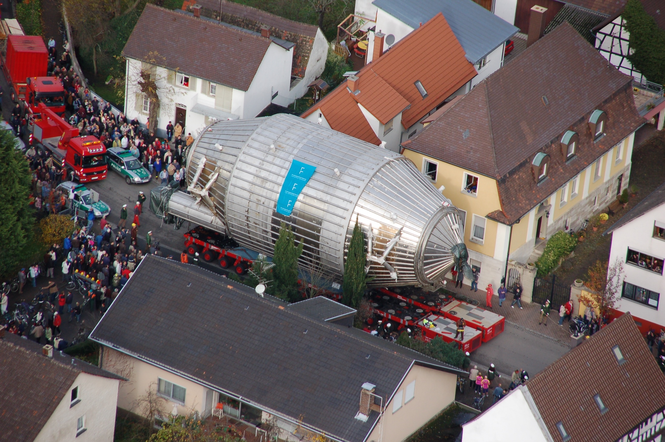
The KATRIN main spectrometer is transported between buildings through Eggenstein-Leopoldshafen

The KATRIN main vessel: length \(23.3\) m, inner diameter \(9.8\) m, mass about \(200\) t. Transport through Eggenstein-Leopoldshafen, 25 November 2006. Photo: Markus Breig, KIT-Archiv 28010/I 7185; source: KIT.

Examples of Magnetic Mirrors

The Van Allen Belts: Earth’s Magnetic Trap

  • 31 January 1958: the first American satellite, Explorer 1, is placed in orbit carrying a Geiger–Müller counter built by James Van Allen’s group.

  • At high altitudes the counter at times showed an almost zero count rate. The cause turned out to be unexpected: the flux was so large that the instrument was saturated.

  • Data from the next satellite, Explorer 3, confirmed a region of intense radiation trapped by the Earth’s magnetic field.

  • The instrument “failure” turned out to be one of the first major discoveries of the space age.

  • The discovery was confirmed by data from the Soviet Sputnik 3.

  • The signal of the radiation belts had also been recorded by the earlier Sputnik 2, but at the time it was not linked to a new region of near-Earth space.

  • The radiation belts are toroidal regions where the magnetic field traps energetic protons and electrons. The particle distribution usually shows two maxima: the inner and outer belts.

Inner Belt

\[ \boxed{h\sim10^3\text{–}1.2\cdot10^4~\mathrm{km}} \]

  • Begins roughly a thousand kilometers above the surface.

  • The most stable; rich in energetic protons.

  • The main source of high-energy protons is the decay of atmospheric neutrons produced by cosmic rays: the CRAND mechanism.

Outer Belt

\[ \boxed{h\sim1.3\cdot10^4\text{–}6\cdot10^4~\mathrm{km}} \]

  • Consists mainly of electrons supplied from the outer magnetosphere.

  • During magnetic storms the electrons are transported and accelerated; the belt can expand, contract, and almost vanish.

The Region Between the Belts

  • Plasmaspheric hiss is electromagnetic oscillations of the plasma that gradually change the direction of motion of electrons. Some of the electrons escape along magnetic field lines into the atmosphere. As a result, a region of reduced electron density forms between the inner and outer radiation belts.

The magnetic mirror explains the trapping of an individual particle, but it does not create two belts. The two maxima arise from different sources, transport, and losses; between them, waves precipitate electrons into the atmosphere especially efficiently.

  • In the inner belt, protons with energies of roughly \(0.1\text{–}400~\mathrm{MeV}\) dominate; electrons of order \(10^2~\mathrm{keV}\) are also present.

  • In the outer belt, electrons of roughly \(0.1\text{–}10~\mathrm{MeV}\) predominate.

  • An electron with kinetic energy \(1~\mathrm{MeV}\) is already relativistic:

\[ \gamma=1+\frac{E}{m_ec^2}\simeq2.96, \qquad v\simeq0.94c. \]

  • These particles damage electronics and solar panels, create background in detectors, and determine the radiation load on spacecraft.

The ranges are approximate: a belt is a broad, variable spectrum, not a beam of particles of a single energy.

Yellow particles are electrons, blue ones are positive ions; the blue-green surface is the plasmapause. NASA/GSFC Scientific Visualization Studio.

  • The particle gyrates around the field line.

  • It bounces between the northern and southern mirror points.

  • It slowly drifts around the Earth.

  • Together these motions fill the toroidal radiation belts.

The spiral is artificially enlarged: on the scale of the whole magnetosphere the individual turns would not be visible.

  • To a first approximation, the Earth's field is a dipole: it is weaker at the equator and grows stronger toward the poles.
  • The particle starts at the equator with a given velocity; the motion of the guiding center is shown, without the cyclotron spiral.
Motion of a particle along a dipole field line of the Earth The interactive shows whether the particle will be reflected by the magnetic mirror or enter the atmosphere, depending on the field line L and the angle between the velocity and the field at the equator. magnetic equator Earth nominal boundary of the atmosphere: 100 km equator: weaker field stronger field toward the poles Field along the chosen line 1 0,5 0 B/Batm south ← s → north mirror: B = Bm Cross section of velocity space v∥ v⊥ red regions are the two loss cones

Problem statement

  • We choose the continuous parameter of the field line L.
  • At the equator we set the angle α between the velocity and the field.
  • We check which comes first for the particle: the mirror point or the atmosphere.

Indices: eq — equator, atm — boundary of the atmosphere.

equatorial altitude heq =
the angle can also be changed with the arrow on the velocity circle
Cone boundary
αloss =
Mirror field
Bm/Batm =
E∥
98%
E⊥
2%
E
100%

  • Consider a dipole field line. \(R_\oplus\) is the Earth’s radius, and \(r_{\mathrm{eq}}\) and \(h_{\mathrm{eq}}\) are the distance from the center and the altitude above the surface at the equator:

\[ L=\frac{r_{\mathrm{eq}}}{R_\oplus}, \qquad h_{\mathrm{eq}}=(L-1)R_\oplus. \]

  • A particle crosses the equator at an angle \(\alpha_{\mathrm{eq}}\) to \(\mathbf B\). From the conservation of \(\mu\) it follows that

\[ B_{\mathrm m} =\frac{B_{\mathrm{eq}}(L)}{\sin^2\alpha_{\mathrm{eq}}}. \]

  • On the same line, the field at the nominal boundary of the atmosphere is \(B_{\mathrm{atm}}(L)\).

\[ \boxed{ \sin^2\alpha_{\mathrm{loss}}(L) =\frac{B_{\mathrm{eq}}(L)}{B_{\mathrm{atm}}(L)} }. \]

Loss cone:

  • For \(\alpha_{\mathrm{eq}}<\alpha_{\mathrm{loss}}(L)\) the particle reaches the atmosphere before the mirror point.

  • For a fixed speed, all directions lie on a sphere in velocity space.

  • Directions with the same angle \(\alpha_{\mathrm{loss}}\) form a circle around the \(\mathbf B\) axis.

  • Smaller angles fill a cone. For the two directions along the field there are two opposite cones.

  • Waves and collisions scatter particles in angle. Once inside the cone, a particle precipitates into the atmosphere.

The field at the equator enters the formula because the initial angle and the magnetic moment of the particle are specified there. Two points on the same line \(L\) are being compared.

More Examples of Magnetic Mirrors

  • The glowing arcs of the solar corona are hot plasma outlining closed magnetic loops.

  • The field strengthens at the footpoints of the loop. Particles with a sufficiently large transverse velocity are reflected and repeatedly travel between the mirror points.

  • Particles from the loss cone reach the chromosphere. Their bremsstrahlung is observed as bright X-ray sources at the footpoints of the flare loop.

  • Mirror confinement affects the duration of solar flares and the distribution of energy between the corona and the lower layers of the atmosphere.
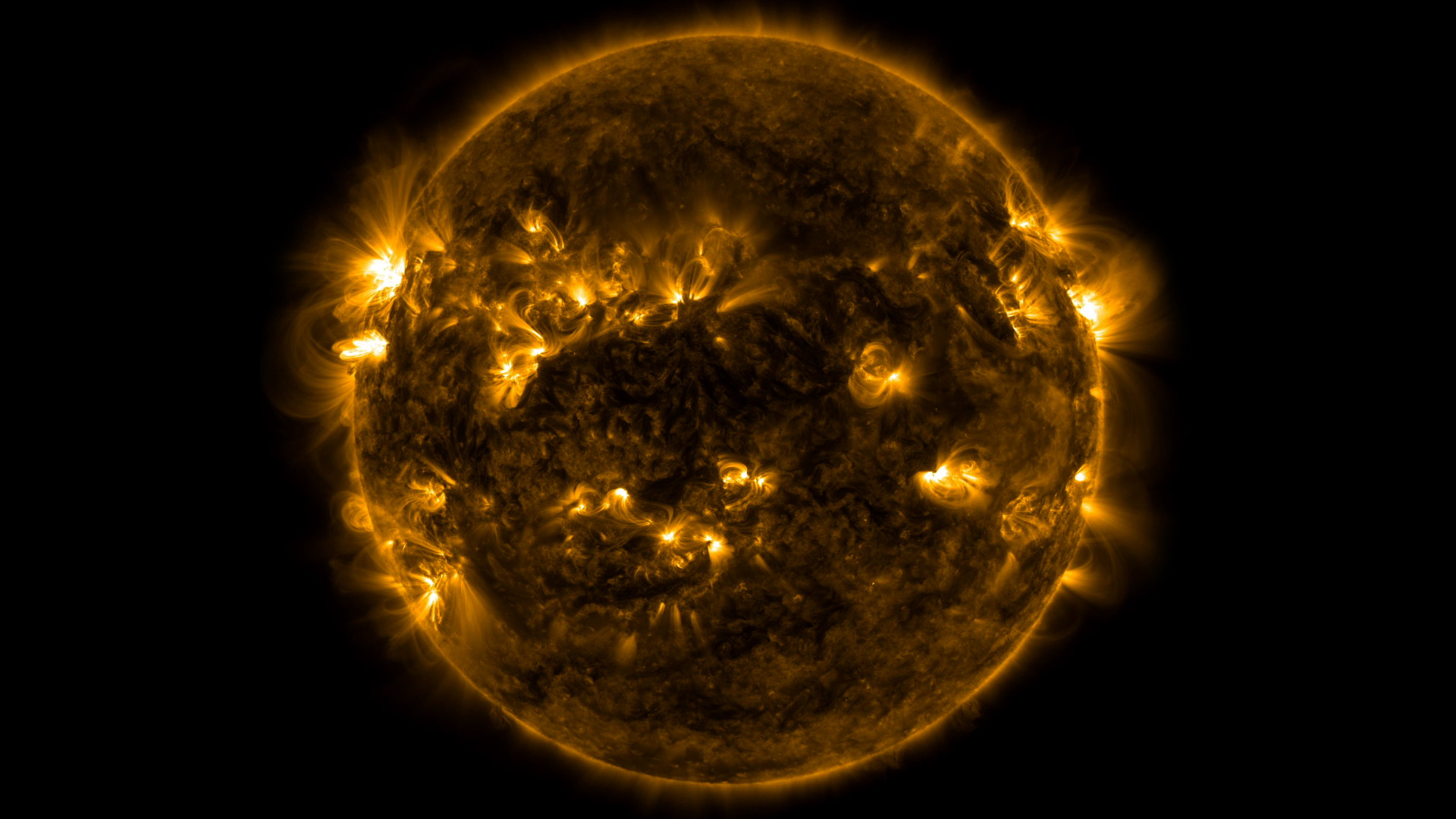
Solar magnetic loops in Solar Dynamics Observatory observations

Hot plasma outlines magnetic loops in the solar corona. NASA/SDO and NASA/GSFC.

  • The main plasma confinement in a tokamak is provided by a toroidal magnetic configuration.

  • The toroidal field is nonuniform:

\[ B(R)\propto\frac{1}{R}. \]

  • On the outer side of the torus the field is weaker, on the inner side stronger. Particles with small \(v_\parallel/v_\perp\) are reflected before reaching the region of maximum field.

  • Together with slow drift, this gives a banana orbit in the poloidal cross-section. Such particles significantly affect neoclassical plasma transport.

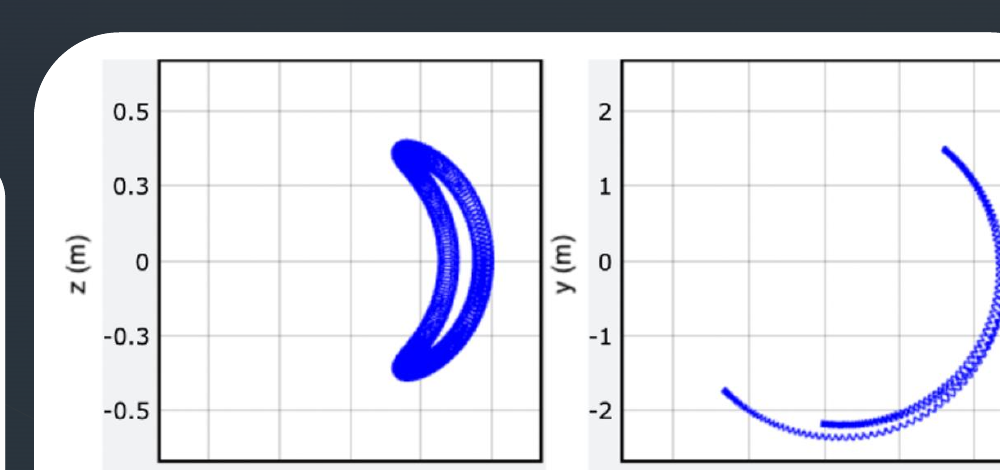
Toroidal surface of the tokamak magnetic field Banana orbit of a trapped particle in a tokamak cross section

Toroidal geometry and the trajectory of a mirror-trapped particle. PPPL educational materials.

  • In an open mirror trap the field is weak in the central chamber and strengthens at the two ends.

  • Particles outside the loss cone are reflected from the magnetic plugs and repeatedly pass through the central plasma.

  • Particles from the loss cone escape through the ends. Reducing these losses is one of the main tasks for mirror fusion devices.

  • Such devices are used in research on controlled fusion, plasma heating, and the interaction of plasma flows with materials.
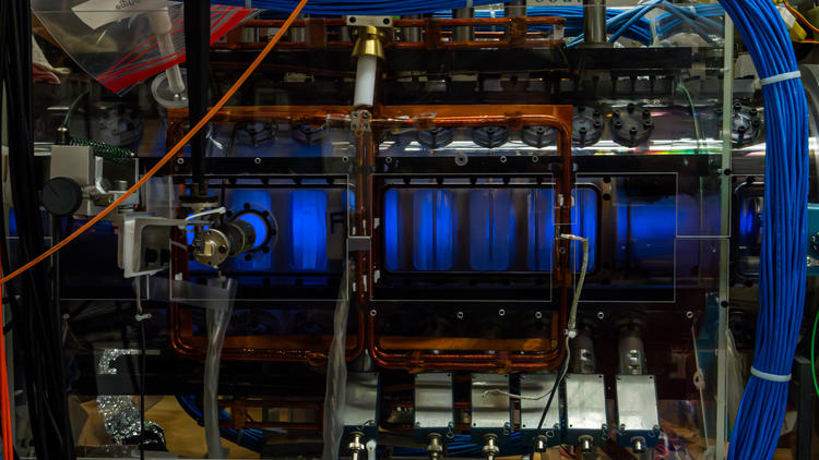
PFRC experimental plasma device at the Princeton Plasma Physics Laboratory

The PFRC experimental device uses magnetic mirrors at its ends. PPPL, 2024.

A particle repeatedly crosses the shock front of a supernova remnant and gains energy. NASA/GSFC.

  • This is how the acceleration of cosmic rays in supernova remnants is explained.
  • In a well-conducting plasma the magnetic field is approximately frozen into the matter. A moving magnetized cloud carries a magnetic inhomogeneity along with it.

  • In the cloud frame the scattering of the particle is almost elastic. In the laboratory frame, a moving magnetic scatterer and the associated electric field can change the particle’s energy.

  • In Fermi’s 1949 model, random clouds give an average gain that is second order in \(u/c\), where \(u\) is the characteristic velocity of the scatterer. Repeated crossings of a shock front give a faster, first-order gain.

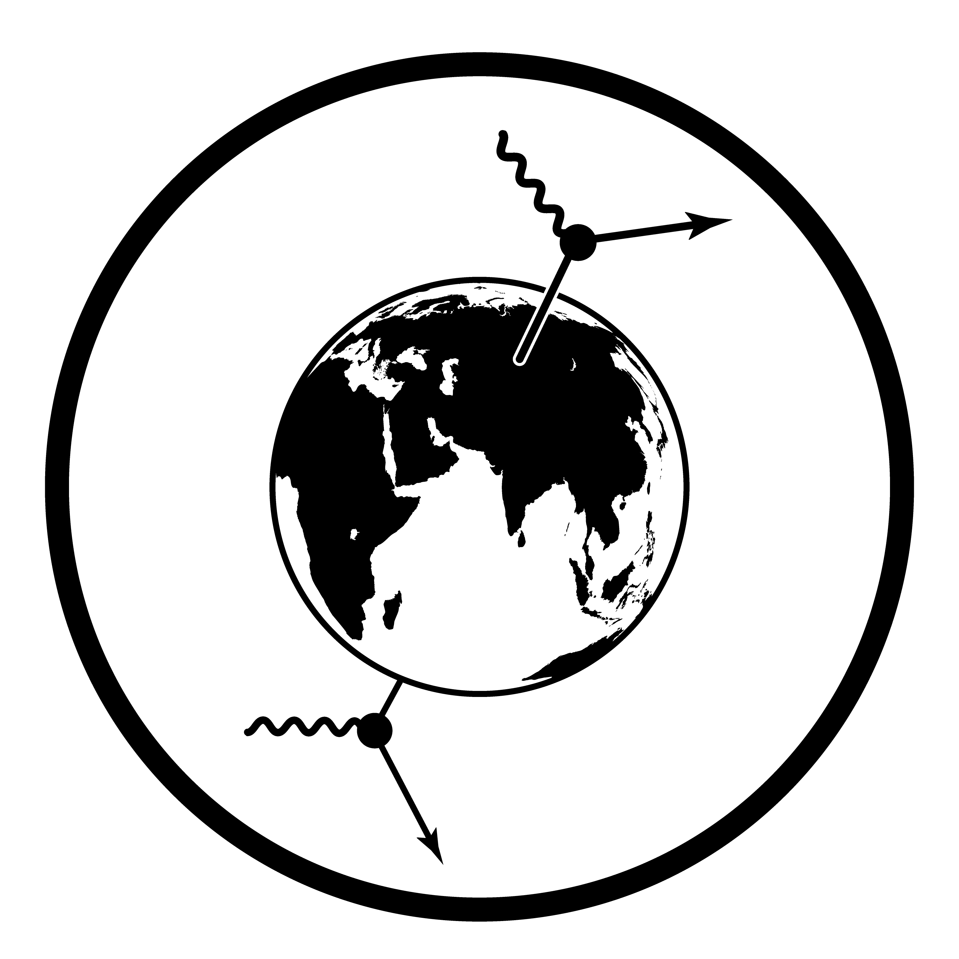
\[ \boxed{ \begin{array}{ll} \text{stationary structure:}&\Delta E=0,\\ \text{moving structure:}&\Delta E\ne0 \end{array} } \]
Summary

Fast and slow motion

\[ T_c\ll\tau_B \quad\Longrightarrow\quad \boxed{J\simeq\mathrm{const}}. \]

After averaging over the fast phase \(\theta\)

\[ \boxed{ \mathcal H_{\mathrm{gc}} =\frac{p_\parallel^2}{2m}+\omega_c(s)J =\frac{p_\parallel^2}{2m}+\mu B(s) }. \]

\[ B\downarrow\Rightarrow\text{collimation}, \qquad B\uparrow\Rightarrow\text{magnetic mirror}. \]

Ideal MAC-E filter

\[ \sin^2\alpha_{\mathrm{acc}} =\frac{B_{\mathrm{src}}}{B_{\max}}, \]

\[ \Delta E =E\frac{B_{\mathrm A}}{B_{\max}}\frac{\gamma+1}{2}, \]

\[ E_{\parallel,\mathrm A} \simeq E-e|U|-E_{\perp,\mathrm A}. \]

\(B_{\mathrm A}\ll B_{\max}\) gives high resolution, but broadens the magnetic tube and requires a huge spectrometer.

We have obtained the transmission of a single electron. In the next lecture, angles, scattering, and source properties will turn the ideal threshold into the response function of the real KATRIN experiment.

Exercises for this lecture

  • 6.1. MAC-E spectrometer numbers
  • 6.2. Two adiabaticity conditions
  • 6.3. Loss cone in a dipole field
  • 6.4. Stationary mirror and Fermi acceleration
  • 6.5. Slow or fast: a numerical test of the invariant
  • 6.6. Magnetic bottle: oscillations between mirrors
  • 6.7. Transmission function of an ideal MAC-E filter
  • 6.8. Why the main spectrometer is the size of a house
  • 6.9. Where is the electron’s fate decided?
  • 6.10. Whom does the Earth’s magnetic field confine?