Direct Determination of the Neutrino Mass. Guiding the Electron to the Detector

Introduction to Neutrino Physics

Dmitry V. Naumov

JINR

Task of the \(\beta\) spectrometer

Integral energy measurement

• The neutrino mass changes the shape of the \(\beta\) spectrum near its endpoint. There are few events there, and the electrons from an unpolarized source are emitted isotropically:

\[ \frac{dN}{d\Omega}=\mathrm{const}. \]

• A small detector looking in only one direction would lose almost all of the statistics.

• Therefore the setup must accept electrons from a large solid angle.

• The energy can be measured integrally. Let us place a retarding electrostatic potential \(U\) in front of the detector:

\[ E<e|U|\ \Longrightarrow\ \text{electron is reflected}, \qquad E>e|U|\ \Longrightarrow\ \text{electron passes through}. \]

When \(U\) is scanned, the detector measures the number of electrons above the threshold:

\[ \boxed{ R(U)\propto \int_{e|U|}^{E_0}\frac{d\Gamma}{dE}\,dE }. \]

Task of the instrument: to collect as many \(\beta\) electrons as possible and compare their energy with a controllable electrostatic threshold.

Longitudinal and transverse motion

• The one-dimensional condition \(E>e|U|\) assumes that the electron moves along the spectrometer axis. In reality its momentum makes an angle \(\alpha\) with the axis:

\[ \mathbf p=\mathbf p_\parallel+\mathbf p_\perp, \qquad E=E_\parallel+E_\perp, \qquad \tan\alpha=\frac{p_\perp}{p_\parallel}. \]

• For the potential \(U(z)\) the transverse momentum is conserved. The longitudinal energy is spent on climbing against the potential, so

\[ \boxed{E_\parallel>e|U|}, \qquad E_\parallel=E\cos^2\alpha \quad\text{(in the nonrelativistic regime)}. \]

• For the same \(E\), electrons with different \(\alpha\) pass different thresholds.

• Keeping only small angles is not an option: the source is isotropic, and the statistics would vanish.

• What is required is a magnetic system that

  1. collects a large solid angle and guides the electrons to the filter;
  2. conserves \(E\);
  3. converts \(E_\perp\) into \(E_\parallel\) before the filter.

Where we are heading

MAC-E: electrons above the threshold pass, electrons below the threshold are reflected.

Uniform magnetic field

Motion in a uniform constant magnetic field

• The main point
• Equation
• Integrals
• Velocity
• Trajectory
• Radius
• Period
• Moment
• Animation

A uniform magnetic field does not change the energy of a particle: it splits the motion into uniform motion along the field and cyclotron rotation transverse to the field.

Conserved

\[ \boxed{p_\parallel=\mathrm{const}}, \qquad \boxed{p_\perp=\mathrm{const}}, \qquad \boxed{E=\mathrm{const}}. \]

Helical trajectory

\[ \boxed{(x-X)^2+(y-Y)^2=\rho_L^2}, \]

\[ \boxed{z(t)=z_0+v_\parallel t}. \]

Over one revolution

\[ \boxed{\omega_c=\frac{|q|B}{m}}, \qquad \boxed{T_c=\frac{2\pi m}{|q|B}}. \]

\[ \boxed{\rho_L=\frac{p_\perp}{|q|B}}, \qquad \boxed{h=\frac{2\pi p_\parallel}{|q|B}}. \]

Orbital magnetic moment

\[ \boxed{ \mu=\frac{E_\perp}{B} =\frac{mv_\perp^2}{2B} =\mathrm{const} }. \]

Relativistic case: \(\omega_c=|q|B/(\gamma m)\), \(T_c=2\pi\gamma m/(|q|B)\); the formulas for \(\rho_L\) and \(h\) in terms of momentum do not change.

Consider a nonrelativistic particle of charge \(q\) and mass \(m\):

\[ \mathbf B=B\mathbf e_z, \qquad \mathbf E=0. \]

The Lorentz force gives

\[ m\dot{\mathbf v} =q\,\mathbf v\times\mathbf B =qB(v_y,-v_x,0), \]

\[ \dot v_x=\Omega v_y, \qquad \dot v_y=-\Omega v_x, \qquad \dot v_z=0. \]

\[ \boxed{\Omega=\frac{qB}{m}}, \qquad \boxed{\omega_c=|\Omega|=\frac{|q|B}{m}}. \]

\(\Omega\) is the signed, and \(\omega_c\) the positive, cyclotron frequency.

The magnetic field does no work:

\[ m\mathbf v\cdot\dot{\mathbf v} = q\mathbf v\cdot(\mathbf v\times\mathbf B) =0. \]

Consequently,

\[ \frac{d}{dt}\frac{mv^2}{2}=0, \qquad v^2=v_\parallel^2+v_\perp^2=\mathrm{const}. \]

Moreover,

\[ v_\parallel=v_z=\mathrm{const}, \qquad v_\perp^2=v_x^2+v_y^2=\mathrm{const}. \]

The field changes the direction of \(\mathbf v_\perp\), but not its magnitude.

\[ \ddot v_x=-\Omega^2v_x, \qquad \ddot v_y=-\Omega^2v_y. \]

Therefore

\[ \boxed{ \begin{aligned} v_x(t) &= v_{x0}\cos\Omega t + v_{y0}\sin\Omega t, \\ v_y(t) &= v_{y0}\cos\Omega t - v_{x0}\sin\Omega t. \end{aligned}} \]

\[ v_x^2(t)+v_y^2(t) = v_{x0}^2+v_{y0}^2 =v_\perp^2. \]

The tip of the vector \(\mathbf v_\perp\) moves along a circle in velocity space.

Integrating the velocity, we obtain

\[ \begin{aligned} x(t) &= x_0+\frac{v_{x0}}{\Omega}\sin\Omega t +\frac{v_{y0}}{\Omega}(1-\cos\Omega t), \\ y(t) &= y_0+\frac{v_{y0}}{\Omega}\sin\Omega t -\frac{v_{x0}}{\Omega}(1-\cos\Omega t), \\ z(t) &= z_0+v_\parallel t. \end{aligned} \]

• In the plane perpendicular to \(\mathbf B\) the particle moves along a circle.

• Along the field the motion is uniform.

\[ \boxed{\Omega=\frac{qB}{m}}, \qquad \boxed{\omega_c=|\Omega|=\frac{|q|B}{m}}. \]

Let us introduce the coordinates of the center of the circle:

\[ \boxed{ X=x+\frac{v_y}{\Omega}, \qquad Y=y-\frac{v_x}{\Omega} }. \]

Using \(\dot v_x=\Omega v_y\) and \(\dot v_y=-\Omega v_x\), we obtain

\[ \dot X=\dot Y=0. \]

Thus \((X,Y)\) is a fixed guiding center, and the distance to it is

\[ \begin{aligned} \rho_L^2 &=(x-X)^2+(y-Y)^2\\ &=\frac{v_x^2+v_y^2}{\Omega^2}. \end{aligned} \]

Hence

\[ \boxed{ \rho_L =\frac{v_\perp}{\omega_c} =\frac{mv_\perp}{|q|B} =\frac{p_\perp}{|q|B} }. \]

Over one revolution the phase changes by \(2\pi\). Therefore

\[ \omega_cT_c=2\pi \quad\Longrightarrow\quad \boxed{T_c=\frac{2\pi m}{|q|B}}. \]

During the same time the guiding center advances along the field by the distance

\[ \boxed{ h=v_\parallel T_c =\frac{2\pi p_\parallel}{|q|B} }. \]

The geometry of the helix directly determines the pitch angle:

\[ \boxed{ \frac{h}{2\pi\rho_L} =\frac{p_\parallel}{p_\perp} =\cot\alpha }. \]

For an electron with \(K=18.6~\mathrm{keV}\) in a field \(B=3.6~\mathrm{T}\), taking \(\gamma=1.036\) into account, we obtain

\[ T_c\simeq10.3~\mathrm{ps}, \qquad \rho_{L,\max}\simeq0.129~\mathrm{mm}. \]

A cyclotron orbit is equivalent to a current loop. The magnitude of the current and the area of the loop are

\[ |I|=\frac{|q|}{T_c}=\frac{|q|\omega_c}{2\pi}, \qquad S=\pi\rho_L^2. \]

Therefore

\[ \begin{aligned} \mu=|I|S &=\frac{|q|\omega_c\rho_L^2}{2}\\ &=\frac{mv_\perp^2}{2B} =\frac{E_\perp}{B}. \end{aligned} \]

The direction of the moment is opposite to the field:

\[ \boxed{ \boldsymbol{\mu}_{\mathrm{orb}}=-\mu\,\mathbf b }, \qquad \mathbf b=\frac{\mathbf B}{B}. \]

In a uniform field \(E_\perp\) and \(B\) are constant, hence

\[ \boxed{\mu=\frac{E_\perp}{B}=\mathrm{const}}. \]

Three electrons are shown at the same moment of time. Their speeds are equal in magnitude, but \(v_z=v\cos\alpha\): a smaller angle gives a larger advance along the field in the same time.

Phase portrait

Three languages

• Newton
• Ellipse
• Lagrange
• Hamilton

• On the previous slides we used the Newtonian formalism to find the electron trajectory in 3D explicitly: \[ \mathbf r(t)=(x(t),y(t),z(t)) \]
• Some properties of a physical system are easier to see on the phase trajectory

\[ (Q(t),P(t)) \]

• For example, for a harmonic oscillator with energy \[ H = \frac{p^2}{2m} + \frac{m\omega^2q^2}{2}=E \] a particular solution is: \[ q(t) = A\cos{\omega t} \]
• In the variables \(q\) and \(p = m\dot{q}\) this is an ellipse

Ordinary space

The displacement from the guiding center changes with time

Phase space

The point moves uniformly around a closed orbit

\[ Q(t)=A\cos\theta, \qquad P(t)=-m\omega A\sin\theta, \qquad \theta=\omega t. \]

• The same particle oscillates in ordinary space and traverses a closed curve in the phase plane.

• Obviously, the area of the ellipse does not change with time. Does it have a physical meaning?

• We will sort this out now!

• The Lagrangian depends on the generalized coordinate \(q\) and the velocity \(\dot{q}\) \[ L(q,\dot{q},t) \]
• Equation of motion: \[ \frac{d}{dt}\frac{\partial L}{\partial \dot{q}}-\frac{\partial L}{\partial q} = 0. \]
• This is a second-order equation

• Let us define the canonical momentum: \[ p\equiv\frac{\partial L}{\partial\dot q} \]
• Hamiltonian

\[ H(q,p,t)\equiv p\dot q-L. \]

• Hamilton’s equations:

\[ \dot q=\frac{\partial H}{\partial p}, \qquad \dot p=-\frac{\partial H}{\partial q}. \]

• These are two first-order equations

Hamiltonian formalism

Phase trajectory

• Constant energy
• Oscillator
• \(J\) (action)
• \(J\) and \((\omega, T)\)
• \(J\) and integrals of motion

If \(H\) does not depend explicitly on time, then

\[ \begin{aligned} \frac{dH}{dt} &=\frac{\partial H}{\partial q}\dot q +\frac{\partial H}{\partial p}\dot p\\ &=-\dot p\dot q+\dot q\dot p=0. \end{aligned} \]

Consequently, the phase point moves along a line of constant energy:

\[ \boxed{H(q,p)=E}. \]

• The phase point \((q,p)\) specifies the state of the system.
• The phase trajectory is a single line \(H=E\).
• The phase portrait is a family of trajectories for different initial conditions.

For a harmonic oscillator

\[ H(q,p)=\frac{p^2}{2m}+\frac{m\omega^2q^2}{2}=E. \]

• The phase trajectories are nested ellipses:

\[ \frac{q^2}{q_{\max}^2}+\frac{p^2}{p_{\max}^2}=1, \]

\[ q_{\max}=\sqrt{\frac{2E}{m\omega^2}}, \qquad p_{\max}=\sqrt{2mE}. \]

• Area of the ellipse: \[ S=\pi q_{\max}p_{\max}=\frac{2\pi E}{\omega}. \]
• Changing \(E\) selects a different ellipse. Changing the parameters \(m\) or \(\omega\) rearranges the whole phase portrait.

Area of the ellipse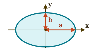

\[ S=\pi ab \]

• So what is the physical meaning of the area of the ellipse in the phase plane?

• Let us define this area via the action \(J\):

\[ \boxed{ J(E)=\frac{1}{2\pi}\oint p\,dq }. \]

• The dimension of \(J\) is that of action, i.e. energy times time.

• The action \(J\) is an integral of motion if the Hamiltonian does not depend explicitly on time:

\[ \boxed{ \dot E=0, \qquad J=J(E) \quad\Longrightarrow\quad \dot J=\frac{dJ}{dE}\dot E=0 }. \]

• A beautiful formula relates the action \(J\) to the period \(T\) and the frequency \(\omega = \frac{2\pi}{T}\): \[ \boxed{\frac{dJ}{dE}=\frac{T}{2\pi} = \frac{1}{\omega}}. \]

• Proof: \[ \begin{aligned} \frac{dJ}{dE} &=\frac{1}{2\pi}\oint \left(\frac{\partial p}{\partial E}\right)_q dq =\frac{1}{2\pi}\oint\frac{dq}{\dot q}\\ &=\frac{1}{2\pi}\int_0^Tdt =\frac{T}{2\pi}=\frac{1}{\omega}. \end{aligned} \]

Four lines

\[ \begin{aligned} H\bigl(q,p\bigr)& =E.\\ \frac{\partial H}{\partial p} \left(\frac{\partial p}{\partial E}\right)_q&=1.\\ \partial H/\partial p&=\dot q,\\ ({\partial p}/{\partial E})_q&=1/\dot q. \end{aligned} \]

• Example: harmonic oscillator \[ J=\frac{1}{2\pi}\pi q_{\max}p_{\max}=\frac{E}{\omega}, \qquad\frac{dJ}{dE} = \frac{1}{\omega}. \]

• \(J\) is an integral of motion.

• For one degree of freedom, \(J\) is not an integral of motion independent of \(E\).

• For \(N>1\) \(J_i\) are integrals of motion independent of \(E\).

Canonical variables

• Change of variables
• Canonical variables

• The same motion can be described by different variables.

• The simplest example is stretching one axis and compressing the other:

\[ Q=aq, \qquad P=\frac{p}{a}. \]

Then

\[ P\,dQ=p\,dq, \]

so the area of the phase orbit does not change.

• A transformation \((q,p)\to(Q,P)\) is called canonical if the Hamilton equations have the same form in the new variables: \[ \dot Q=\frac{\partial H}{\partial P},\qquad \dot P=-\frac{\partial H}{\partial Q}. \]

• A canonical transformation can stretch and deform the phase plane, but it preserves the oriented area: \[ dq\,dp=dQ\,dP. \]

• Strictly, this is written through the symplectic form:

\[ dq\wedge dp=dQ\wedge dP, \]

• Then,

\[ \oint p\,dq = \oint P\,dQ. \]

Cyclotron orbit in the variables \((\theta,J)\)

• \((Q,P)\)
• \(J\)
• \(\theta\)
• Poisson bracket
• Equations of motion
• From \((\mathbf r,\mathbf p)\) to \((J,\theta)\)
• Portrait

Hamilton’s equations

\[ \dot Q=\frac{\partial H}{\partial P}, \qquad \dot P=-\frac{\partial H}{\partial Q}. \]

• Let us separate the motion relative to the guiding center. For \(\Omega=qB/m\) and \(\omega_c=|\Omega|\) we introduce

\[ Q\equiv x-X=-\frac{v_y}{\Omega}, \qquad P\equiv m\dot Q=mv_x. \]

• Then the cyclotron equations take the form

\[ \dot Q=\frac{P}{m}, \qquad \dot P=-m\omega_c^2Q. \]

• These are the Hamilton equations for the oscillator

\[ \boxed{ H_\perp(Q,P) =\frac{P^2}{2m}+\frac{m\omega_c^2Q^2}{2} =E_\perp }. \]

Thus \((Q,P)\) is a canonical pair for one periodic degree of freedom.

• Let us apply the already introduced definition of the action to the ellipse \(H_\perp(Q,P)=E_\perp\):

\[ \boxed{ J\equiv\frac{1}{2\pi}\oint P\,dQ =\frac{E_\perp}{\omega_c} }. \]

• Therefore \(J\):

\[ \boxed{ J(Q,P) =\frac{H_\perp(Q,P)}{\omega_c} =\frac{P^2}{2m\omega_c}+\frac{m\omega_cQ^2}{2} }. \]

• \(J\) determines which ellipse is chosen. But where is the particle on it?

• We specify the position on the chosen ellipse by the angle

\[ \boxed{ \theta(Q,P) =\operatorname{atan2}\!\left(m\omega_cQ,\,P\right) }. \]

\(\operatorname{atan2}(y,x)\) is the ordinary polar angle of the point \((x,y)\) with the correct choice of quadrant. Here it is the angle of the point \((P,m\omega_cQ)\).

• Together, the definitions \(J(Q,P)\) and \(\theta(Q,P)\) give the inverse change of variables

\[ Q=\sqrt{\frac{2J}{m\omega_c}}\sin\theta, \qquad P=\sqrt{2m\omega_cJ}\cos\theta. \]

\(J\) specifies the ellipse, and \(\theta\) the position of the phase point on it. At the center \(J=0\) the angle is undefined, since the orbit itself degenerates into a point.

• For functions of the phase variables the Poisson bracket is defined as

\[ \boxed{ \{f,g\}_{Q,P} \equiv \frac{\partial f}{\partial Q}\frac{\partial g}{\partial P} -\frac{\partial f}{\partial P}\frac{\partial g}{\partial Q} }. \]

• Substituting the found \(\theta(Q,P)\) and \(J(Q,P)\), we obtain

\[ \begin{gathered} D\equiv P^2+(m\omega_cQ)^2,\\ \frac{\partial\theta}{\partial Q}=\frac{m\omega_cP}{D}, \qquad \frac{\partial\theta}{\partial P}=-\frac{m\omega_cQ}{D},\\ \frac{\partial J}{\partial P}=\frac{P}{m\omega_c}, \qquad \frac{\partial J}{\partial Q}=m\omega_cQ. \end{gathered} \]

\[ \boxed{ \{\theta,J\}_{Q,P} =\frac{P^2+(m\omega_cQ)^2} {P^2+(m\omega_cQ)^2} =1 }. \]

For one pair, \(\{\theta,J\}=1\) is the condition of canonicity (\(\{\theta,\theta\}=\{J,J\}=0\) holds automatically). Therefore \(\theta\) is the coordinate, \(J\) is the conjugate momentum, and the Hamilton equations keep their form.

• In the variables \((\theta,J)\) the Hamiltonian does not depend on the angle:

\[ \boxed{H_\perp=\omega_cJ}, \qquad \frac{\partial H_\perp}{\partial\theta}=0. \]

• Since \((\theta,J)\) is a canonical pair,

\[ \dot\theta=\frac{\partial H_\perp}{\partial J}, \qquad \dot J=-\frac{\partial H_\perp}{\partial\theta}. \]

• From this directly

\[ \boxed{\dot\theta=\omega_c}, \qquad \boxed{\dot J=0}. \]

\(J\) remains constant, and the phase point goes around the chosen orbit uniformly: \(\theta(t)=\theta_0+\omega_ct\).

• The full state of a particle in three-dimensional space is given by six numbers \((\mathbf r,\mathbf p)\):

\[ \boxed{ (\mathbf r,\mathbf p) \ \longleftrightarrow\ \underbrace{(X,Y)}_{\substack{\text{guiding}\\\text{center}}} \oplus \underbrace{(z,p_\parallel)}_{\substack{\text{motion}\\\text{along the field}}} \oplus \underbrace{(Q,P)}_{\substack{\text{cyclotron}\\\text{motion}}} }. \]

• In a uniform field

\[ \dot X=\dot Y=\dot p_\parallel=0, \qquad \dot z=\frac{p_\parallel}{m}. \]

• What remains are \(z,Q,P\): the coordinate \(z\) grows uniformly, while the point \((Q,P)\) moves along a closed orbit.

• For cyclotron motion we replace one canonical pair by another:

\[ \boxed{(Q,P)\ \longleftrightarrow\ (\theta,J)}, \qquad \boxed{\{\theta,J\}=1}. \]

• \(J\) selects the orbit. The coordinate \(\theta\) conjugate to it specifies the position of the particle on this orbit.

Transverse energy, E⊥/E₀

1,00

Magnetic field, B/B₀

1,00

Semi-axis along Q: ∝ √E⊥/B

Semi-axis along P: ∝ √E⊥

Phase-space area: 2πJ

J/J₀: 1,00

The many faces of the action \(J\)

• Cyclotron orbit
• Planar rotator
• Action of the rotator
• The angle \(\theta\)
• Pendulum

Recall

\[ \omega_c=\frac{|q|B}{m} \]

Recall

\[ \rho_L=\frac{p_\perp}{|q|B} \]

• For cyclotron motion the action is:

\[ \boxed{ J =\frac{1}{2\pi}\oint P\,dQ =\frac{E_\perp}{\omega_c} =\frac{p_\perp^2}{2|q|B} }. \]

• For a circular cyclotron orbit the action \(J\) is related:
  • to the orbital angular momentum \(L_{\mathrm{orb}}\equiv|\mathbf L_{\mathrm{orb}}|=\rho_Lp_\perp\): \[ J=\frac{L_{\mathrm{orb}}}{2}. \]
  • to the orbital magnetic moment \(\mu=\frac{|q|L_{\mathrm{orb}}}{2m}\): \[ J = \frac{m}{|q|}\mu. \]
  • to the magnetic flux \(\Phi=\pi\rho_L^2B\) through the area of the orbit: \[ J=\frac{|q|}{2\pi}\Phi \]

• A bead of mass \(m\) is fixed at the end of a massless rigid rod of length \(R\).

• The point \(O\) is fixed; the rod rotates without friction in a horizontal plane.

• This is a planar rotator.

• The radius is fixed, so one coordinate remains — the angle \(\varphi\):

\[ I=mR^2, \qquad \mathcal L=\frac{I\dot\varphi^2}{2}, \qquad p_\varphi=\frac{\partial\mathcal L}{\partial\dot\varphi} =I\dot\varphi=L_z. \]

• The angle \(\varphi\) does not enter \(\mathcal L\), so it is cyclic and \(p_\varphi\) is conserved.

• The Hamiltonian has the form

\[ H=\frac{p_\varphi^2}{2I}, \qquad \dot p_\varphi=0. \]

φ = 0.00 rad R = const ω = const

The rod fixes a constant radius; the constraint force is directed toward point O and produces no torque about O.

• Consider rotation in a chosen direction, for example \(p_\varphi>0\). On this branch \(p_\varphi\) is constant, and in one revolution \(\varphi\) increases by \(2\pi\):

\[ \begin{aligned} J &=\frac{1}{2\pi}\oint p_\varphi\,d\varphi \\ &=\frac{1}{2\pi} \int_{\varphi_0}^{\varphi_0+2\pi}p_\varphi\,d\varphi =p_\varphi=L_z. \end{aligned} \]

• In general the action is chosen to be positive:

\[ \boxed{J=|p_\varphi|=|L_z|}. \]

• For the branch \(p_\varphi>0\) the conjugate angle is the coordinate \(\theta=\varphi\) itself. Indeed,

\[ \{\theta,J\}=\{\varphi,p_\varphi\}=1, \qquad H(J)=\frac{J^2}{2I}. \]

• The Hamilton equations give uniform rotation:

\[ \boxed{ \dot\theta=\frac{\partial H}{\partial J}=\frac{J}{I}=\omega, \qquad \dot J=-\frac{\partial H}{\partial\theta}=0 }. \]

• \(J\) indicates which rotation is chosen: its angular momentum and energy;
• \(\theta\) indicates where the bead is within the revolution.

For the rotator the action coincided with the magnitude of the angular momentum. This is a special result; the definition \(J=(2\pi)^{-1}\oint p\,dq\) remains the general one.

For the pendulum the spatial motion goes back and forth, but in the phase plane \((\varphi,p_\varphi)\) an oscillation corresponds to a closed curve.

For each oscillatory regime we obtain its own orbit:

\[ H(\varphi,p_\varphi)=E, \qquad J(E)=\frac{1}{2\pi}\oint p_\varphi\,d\varphi. \]

The pendulum orbit is no longer an ellipse, yet its phase area still provides a label of the periodic motion. The definition \(J\) works for any closed phase trajectory.

Summary

The spectrometer measures the longitudinal energy

\[ \boxed{E_\parallel>e|U|}. \]

The magnetic system must collect a large solid angle, guide the electrons to the filter, and before it convert \(E_\perp\) into \(E_\parallel\) at \(E=\mathrm{const}\).

Uniform magnetic field

\[ \begin{gathered} E=\mathrm{const}, \qquad p_\parallel=\mathrm{const}, \qquad p_\perp=\mathrm{const},\\[0.4em] \rho_L=\frac{p_\perp}{|q|B}, \qquad \omega_c=\frac{|q|B}{m}. \end{gathered} \]

\[ \tan\alpha=\frac{p_\perp}{p_\parallel}=\mathrm{const} \]

The trajectory is helical, the guiding center is stationary. The field guides the electron but does not collimate the beam.

One periodic degree of freedom

\[ J=\frac{1}{2\pi}\oint p\,dq \qquad \frac{dJ}{dE}=\frac{1}{\omega} \]

\(2\pi J\) is the area inside the closed phase orbit.

Cyclotron motion

\[ J=\frac{E_\perp}{\omega_c} =\frac{p_\perp^2}{2|q|B} =\frac{m}{|q|}\mu \]

\[ (Q,P)\longleftrightarrow(\theta,J), \qquad \{\theta,J\}=1 \]

\[ H_\perp=\omega_cJ, \qquad \dot J=0, \qquad \dot\theta=\omega_c \]

\(J\) specifies the cyclotron orbit; \(\theta\) is the position of the particle on it.

\(J\) will become the central quantity in the method of adiabatic collimation.

Exercises for this lecture

• 5.1. Time of flight along a helical trajectory
• 5.2. Electrostatic threshold and angular acceptance
• 5.3. Guiding center and the sign of the charge
• 5.4. From the phase ellipse to the variables \((\theta,J)\)
• 5.5. Four physical meanings of the action

• 5.6. Relativistic transverse energy
• 5.7. Period from area: a box and a bouncing ball
• 5.8. Which changes of variables are canonical?
• 5.9. The pendulum: from oscillation to rotation

All exercises for lecture 05 → and exercises for the seminar · All course exercises