viewof fermiMass = Inputs.range([0, 3], {
  value: 1,
  step: 0.1,
  label: html`
    <span class="spectrum-slider-label">
      ${tex`m_\nu,\ \text{eV}`}
    </span>
  `
})

fermiElectronMass = 511000
fermiEndpoint = 18575
fermiWindow = 3

fermiSpectrum = (energy, mass) => {
  const neutrinoEnergy = fermiEndpoint - energy;
  if (neutrinoEnergy < mass) return 0;
  const electronMomentum = Math.sqrt(
    energy * energy + 2 * fermiElectronMass * energy
  );
  const neutrinoMomentum = Math.sqrt(Math.max(
    0,
    neutrinoEnergy * neutrinoEnergy - mass * mass
  ));
  return electronMomentum
    * (energy + fermiElectronMass)
    * neutrinoEnergy
    * neutrinoMomentum;
}

fermiIntegrate = (lower, upper, mass, steps = 1000) => {
  if (upper <= lower) return 0;
  const step = (upper - lower) / steps;
  let sum = (
    fermiSpectrum(lower, mass)
    + fermiSpectrum(upper, mass)
  ) / 2;
  for (let i = 1; i < steps; i += 1) {
    sum += fermiSpectrum(lower + i * step, mass);
  }
  return sum * step;
}

fermiNorm = fermiSpectrum(fermiEndpoint - fermiWindow, 0)
fermiTotalIntegral = fermiIntegrate(0, fermiEndpoint, 0, 8000)
fermiShadedIntegral = fermiIntegrate(
  fermiEndpoint - fermiMass,
  fermiEndpoint,
  0,
  400
)
fermiShadedFraction = fermiShadedIntegral / fermiTotalIntegral
fermiFractionExponent = fermiShadedFraction === 0
  ? 0
  : Math.floor(Math.log10(fermiShadedFraction))
fermiFractionMantissa = fermiShadedFraction === 0
  ? "0"
  : (
    fermiShadedFraction / 10 ** fermiFractionExponent
  ).toFixed(2)

fermiX = Array.from({length: 501}, (_, i) =>
  -fermiWindow + fermiWindow * i / 500
)
fermiMassless = fermiX.map(x => ({
  x,
  y: fermiSpectrum(fermiEndpoint + x, 0) / fermiNorm
}))
fermiMassive = fermiX
  .filter(x => -x >= fermiMass)
  .map(x => ({
    x,
    y: fermiSpectrum(fermiEndpoint + x, fermiMass) / fermiNorm
  }))
fermiShaded = fermiMassless.filter(d => d.x >= -fermiMass)

fermiPlot = Plot.plot({
  width: 1120,
  height: 300,
  marginTop: 18,
  marginRight: 25,
  marginBottom: 45,
  marginLeft: 72,
  style: {
    background: "#ffffff",
    color: "#111111",
    fontSize: "20px"
  },
  x: {
    axis: "bottom",
    label: null,
    domain: [-fermiWindow, 0],
    ticks: 6,
    grid: true
  },
  y: {
    axis: "left",
    label: null,
    domain: [0, 1.05],
    ticks: 5,
    grid: true,
    tickFormat: value => value.toFixed(1)
  },
  marks: [
    Plot.areaY(fermiShaded, {
      x: "x",
      y: "y",
      fill: "#999999",
      fillOpacity: 0.65
    }),
    Plot.ruleY([0], {
      stroke: "#111111",
      strokeWidth: 1.5
    }),
    Plot.line(fermiMassless, {
      x: "x",
      y: "y",
      stroke: "#4ea1ff",
      strokeWidth: 4
    }),
    Plot.line(fermiMassive, {
      x: "x",
      y: "y",
      stroke: "#ffb347",
      strokeWidth: 4
    }),
    Plot.ruleX([-fermiMass], {
      stroke: "#ffb347",
      strokeDasharray: "7,5",
      strokeWidth: 2.5
    }),
    Plot.frame({stroke: "#111111"})
  ]
})

html`
<div class="spectrum-panel">
  <div class="spectrum-legend">
    <span>
      <i class="spectrum-swatch spectrum-swatch-massless"></i>
      ${tex`m_\nu=0`}
    </span>
    <span>
      <i class="spectrum-swatch spectrum-swatch-massive"></i>
      ${tex`m_\nu=${fermiMass.toFixed(1)}\ \mathrm{eV}`}
    </span>
  </div>
  <div class="spectrum-plot-row">
    <div class="spectrum-y-label">
      ${tex`\dfrac{d\Gamma}{dE}\;(\mathrm{a.u.})`}
    </div>
    <div class="spectrum-plot-host">
      ${fermiPlot}
      <div class="spectrum-integral-overlay">
        <span>
          ${tex`\dfrac{\int_{E_0-m_\nu}^{E_0}(d\Gamma/dE)\,dE}
          {\int_0^{E_0}(d\Gamma/dE)\,dE}`}
        </span>
        <span>
          ≈ ${fermiFractionMantissa}
          ${fermiShadedFraction === 0
            ? ""
            : html`× 10<sup>${fermiFractionExponent}</sup>`}
        </span>
      </div>
    </div>
  </div>
  <div class="spectrum-x-label">
    ${tex`E-E_0\;(\mathrm{eV})`}
  </div>
  <div class="spectrum-summary">
    <span>${tex`E_0=18.575\ \mathrm{keV}`}</span>
    <span>${tex`E_{\max}=E_0-m_\nu`}</span>
  </div>
</div>`Direct Determination of the Neutrino Mass. Kinematics of the β Spectrum
Introduction to Neutrino Physics
Dmitry V. Naumov
JINR
Neutrinos Have Mass
Neutrinos Have Nonzero Mass
- Neutrino oscillations are reliably observed. Therefore \[ \Delta m^2_{ij}\ne 0. \]
- The neutrino mass is nonzero, and also \(m_i\ne m_j\).
- How can we measure the masses themselves, rather than the differences of squared masses?
Method for Measuring the Neutrino Mass in \(\beta\) Decays
- The idea of measuring the shape of the \(\beta\) spectrum to determine the neutrino mass was proposed by Perrin (1933) and Fermi (1934)
- The first experiments using this method were performed by Curran, Angus, and Cockcroft (1948) and by Hanna and Pontecorvo (1949)
The Essence of the Method
For a single neutrino mass state:
\[ \frac{d\Gamma}{dE} \propto \underbrace{F(Z,E)}_{\substack{\text{Coulomb}\\\text{correction}}}\, \underbrace{\sqrt{E^2+2m_eE}}_{p_e}\, \underbrace{(E+m_e)}_{E_e}\, \underbrace{(E_0-E)}_{E_\nu}\, \underbrace{\sqrt{(E_0-E)^2-m_\nu^2}}_{p_\nu}\, \Theta(E_0-E-m_\nu), \]
where \(E\) is the kinetic energy of the electron, and \(E_0\) is the maximum possible electron energy subject to \(m_\nu=0\).
The Fermi Function \(F(Z,E;A)\)
For free particles it is convenient to compute the spectrum with plane waves. For the neutrino this is a good approximation, but the charged lepton is born inside the Coulomb field of the daughter nucleus. Therefore a plane electron wave is not a state of the final Hamiltonian:
\[ \left[ \boldsymbol\alpha\cdot\mathbf p+\beta m_e+V_C(r) \right]\psi^{(-)}_{E_e\mathbf p}(\mathbf r) =E_e\psi^{(-)}_{E_e\mathbf p}(\mathbf r), \qquad V_C(r)\simeq-\frac{Z_d\alpha}{r}. \]
For an allowed transition, \(p_eR\ll1\) and \(p_\nu R\ll1\), the weak vertex probes the electron wave in the region of the nucleus:
\[ \mathcal M_{fi}\simeq \psi_{E_e\mathbf p}^{(-)*}(R)\,\mathcal M_{\mathrm{nucl}}, \qquad \boxed{ F(Z_d,E_e;A)= \frac{|\psi_C^{(-)}(R)|^2}{|\psi_{\mathrm{pw}}(R)|^2} }. \]
That is, the simple result is not discarded but multiplied by the calculable ratio of wave densities in the region of the weak vertex:
\[ \boxed{ \frac{d\Gamma_C}{dE_e} =F(Z_d,E_e;A)\frac{d\Gamma_{\mathrm{pw}}}{dE_e} }. \]
\(F\) is not a phenomenological “energy loss after the decay”: it corrects the matrix element, not the neutrino phase space.
Let us reverse the picture in time: a slow electron with a given asymptotic momentum falls onto a positive nucleus. The attraction increases the density of its wave at the nucleus. Therefore for \(\beta^-\) decay
\[ \eta=\frac{Z_d\alpha}{\beta_e}, \qquad \boxed{ F_{\mathrm{NR}}(Z_d,E_e) =\frac{2\pi\eta}{1-e^{-2\pi\eta}}>1 }, \qquad \beta_e=\frac{p_e}{E_e}. \]
For \(\beta_e\ll1\) we have \(F_{\mathrm{NR}}\simeq2\pi Z_d\alpha/\beta_e\): this is the Sommerfeld Coulomb enhancement. For \(\beta^+\) the sign of the potential changes, the wave is defocused, and \(F<1\).
For an allowed transition and \(m_\nu=0\):
\[ \frac{d\Gamma_\mp}{dK}\propto F(\pm Z_d,E_e;A)\,p_eE_e(E_0-K)^2, \qquad E_e=K+m_e. \]
viewof fermiCompareParameters = {
  const control = html`<div class="fermi-compare-controls">
    <label>
      <span>${tex`Z_d`}</span>
      <output></output>
      <input name="charge" type="range"
        min="1" max="60" step="1" value="29">
    </label>
    <label>
      <span>${tex`A`}</span>
      <output></output>
      <input name="massNumber" type="range"
        min="2" max="160" step="1" value="64">
    </label>
    <label>
      <span>${tex`E_0,\ \text{MeV}`}</span>
      <output></output>
      <input name="endpoint" type="range"
        min="0.5" max="4" step="0.1" value="2">
    </label>
  </div>`;

  const inputs = [...control.querySelectorAll("input")];
  const outputs = [...control.querySelectorAll("output")];

  function update(dispatch = true) {
    control.value = {
      charge: Number(inputs[0].value),
      massNumber: Number(inputs[1].value),
      endpoint: Number(inputs[2].value)
    };
    outputs[0].textContent = String(control.value.charge);
    outputs[1].textContent = String(control.value.massNumber);
    outputs[2].textContent = control.value.endpoint.toFixed(1);
    if (dispatch) {
      control.dispatchEvent(new Event("input", {bubbles: true}));
    }
  }

  inputs.forEach(input => input.addEventListener("input", () => update()));
  update(false);
  return control;
}

fermiCompareAlpha = 1 / 137.035999084
fermiCompareElectronMass = 510.99895
fermiCompareHbarC = 197326.9804
fermiCompareLanczos = [
  676.5203681218851,
  -1259.1392167224028,
  771.3234287776531,
  -176.6150291621406,
  12.507343278686905,
  -0.13857109526572012,
  9.984369578019572e-6,
  1.5056327351493116e-7
]

fermiCompareComplexAdd = (a, b) => ({
  re: a.re + b.re,
  im: a.im + b.im
})

fermiCompareComplexMultiply = (a, b) => ({
  re: a.re * b.re - a.im * b.im,
  im: a.re * b.im + a.im * b.re
})

fermiCompareRealDivide = (a, b) => {
  const denominator = b.re * b.re + b.im * b.im;
  return {
    re: a * b.re / denominator,
    im: -a * b.im / denominator
  };
}

fermiCompareComplexLog = z => ({
  re: Math.log(Math.hypot(z.re, z.im)),
  im: Math.atan2(z.im, z.re)
})

fermiCompareLogGamma = z => {
  const shifted = {re: z.re - 1, im: z.im};
  let series = {re: 0.9999999999998099, im: 0};
  fermiCompareLanczos.forEach((coefficient, index) => {
    series = fermiCompareComplexAdd(
      series,
      fermiCompareRealDivide(coefficient, {
        re: shifted.re + index + 1,
        im: shifted.im
      })
    );
  });
  const t = {re: shifted.re + 7.5, im: shifted.im};
  const power = fermiCompareComplexMultiply(
    {re: shifted.re + 0.5, im: shifted.im},
    fermiCompareComplexLog(t)
  );
  return fermiCompareComplexAdd(
    {re: 0.5 * Math.log(2 * Math.PI) - t.re, im: -t.im},
    fermiCompareComplexAdd(power, fermiCompareComplexLog(series))
  );
}

fermiCompareFactor = (charge, massNumber, kineticEnergy, leptonSign) => {
  const totalEnergy = kineticEnergy + fermiCompareElectronMass;
  const momentum = Math.sqrt(
    kineticEnergy * (kineticEnergy + 2 * fermiCompareElectronMass)
  );
  const gamma = Math.sqrt(1 - (charge * fermiCompareAlpha) ** 2);
  const eta = leptonSign * charge * fermiCompareAlpha
    * totalEnergy / momentum;
  const radius = 1.2 * massNumber ** (1 / 3) / fermiCompareHbarC;
  const logGammaReal = fermiCompareLogGamma({
    re: 2 * gamma + 1,
    im: 0
  }).re;
  const logGammaComplex = fermiCompareLogGamma({
    re: gamma,
    im: eta
  }).re;
  const logFactor = Math.log(2 * (1 + gamma))
    - 2 * logGammaReal
    + 2 * (gamma - 1) * Math.log(2 * momentum * radius)
    + Math.PI * eta
    + 2 * logGammaComplex;
  return Math.exp(logFactor);
}

fermiCompareEndpoint = 1000 * fermiCompareParameters.endpoint

fermiComparePlaneRate = kineticEnergy => {
  const totalEnergy = kineticEnergy + fermiCompareElectronMass;
  const momentum = Math.sqrt(
    kineticEnergy * (kineticEnergy + 2 * fermiCompareElectronMass)
  );
  const neutrinoEnergy = fermiCompareEndpoint - kineticEnergy;
  return momentum * totalEnergy * neutrinoEnergy * neutrinoEnergy;
}

fermiCompareKineticEnergies = Array.from({length: 601}, (_, index) =>
  Math.max(0.05, fermiCompareEndpoint * index / 600)
).filter(energy => energy < fermiCompareEndpoint)

fermiCompareRaw = leptonSign => fermiCompareKineticEnergies.map(energy => {
  const plane = fermiComparePlaneRate(energy);
  const factor = fermiCompareFactor(
    fermiCompareParameters.charge,
    fermiCompareParameters.massNumber,
    energy,
    leptonSign
  );
  return {energy: energy / 1000, plane, corrected: factor * plane};
})

fermiCompareNormalize = data => {
  const planeMaximum = Math.max(...data.map(d => d.plane));
  const correctedMaximum = Math.max(...data.map(d => d.corrected));
  return data.map(d => ({
    energy: d.energy,
    plane: d.plane / planeMaximum,
    corrected: d.corrected / correctedMaximum
  }));
}

fermiCompareMinusData = fermiCompareNormalize(fermiCompareRaw(1))
fermiComparePlusData = fermiCompareNormalize(fermiCompareRaw(-1))

fermiComparePlot = (data, color) => Plot.plot({
  width: 840,
  height: 370,
  marginTop: 10,
  marginRight: 18,
  marginBottom: 50,
  marginLeft: 62,
  style: {
    background: "#ffffff",
    color: "#111111",
    fontSize: "22px"
  },
  x: {
    axis: "bottom",
    label: "K (MeV)",
    domain: [0, fermiCompareParameters.endpoint],
    ticks: 5,
    grid: true
  },
  y: {
    axis: "left",
    label: null,
    domain: [0, 1.05],
    ticks: 5,
    grid: true,
    tickFormat: value => value.toFixed(1)
  },
  marks: [
    Plot.areaY(data, {
      x: "energy",
      y: "corrected",
      fill: color,
      fillOpacity: 0.14
    }),
    Plot.line(data, {
      x: "energy",
      y: "plane",
      stroke: "#777777",
      strokeWidth: 2.5,
      strokeDasharray: "7,5"
    }),
    Plot.line(data, {
      x: "energy",
      y: "corrected",
      stroke: color,
      strokeWidth: 4
    }),
    Plot.frame({stroke: "#111111"})
  ]
})

fermiCompareMinusPlot = fermiComparePlot(
  fermiCompareMinusData,
  "#4ea1ff"
)
fermiComparePlusPlot = fermiComparePlot(
  fermiComparePlusData,
  "#ffb347"
)

fermiCompareProbeEnergy = Math.min(10, 0.02 * fermiCompareEndpoint)
fermiCompareMinusProbe = fermiCompareFactor(
  fermiCompareParameters.charge,
  fermiCompareParameters.massNumber,
  fermiCompareProbeEnergy,
  1
)
fermiComparePlusProbe = fermiCompareFactor(
  fermiCompareParameters.charge,
  fermiCompareParameters.massNumber,
  fermiCompareProbeEnergy,
  -1
)

html`<div class="fermi-compare-grid">
  <div class="fermi-compare-panel">
    <div class="fermi-compare-title">
      ${tex`\beta^-:`} attraction to the nucleus
    </div>
    <div class="spectrum-plot-host">${fermiCompareMinusPlot}</div>
    <div class="fermi-compare-readout">
      ${tex`F(+Z_d,K=${fermiCompareProbeEnergy.toFixed(0)}\,\mathrm{keV})
      =${fermiCompareMinusProbe.toFixed(2)}`}
    </div>
  </div>
  <div class="fermi-compare-panel">
    <div class="fermi-compare-title">
      ${tex`\beta^+:`} repulsion from the nucleus
    </div>
    <div class="spectrum-plot-host">${fermiComparePlusPlot}</div>
    <div class="fermi-compare-readout">
      ${tex`F(-Z_d,K=${fermiCompareProbeEnergy.toFixed(0)}\,\mathrm{keV})
      =${fermiComparePlusProbe.toFixed(2)}`}
    </div>
  </div>
</div>
<div class="fermi-compare-note">
  <span class="fermi-line-key fermi-line-key-plane"></span>
  plane wave;
  <span class="fermi-line-key" style="color:#b8d9ff"></span>
  with ${tex`F(\pm Z_d,E_e;A)`}.<br>
  Each curve is normalized to its own maximum; identical parameters isolate
  the pure effect of the sign of the charge.
</div>`
For a point nucleus, the solution of the Dirac equation gives
\[ \boxed{ F_0(Z_d,E_e;R)= \frac{2(1+\gamma)}{\Gamma(2\gamma+1)^2} (2p_eR)^{2(\gamma-1)} e^{\pi\eta}|\Gamma(\gamma+i\eta)|^2 }, \]
\[ \gamma=\sqrt{1-(Z_d\alpha)^2}, \qquad \eta=\frac{Z_d\alpha E_e}{p_e}, \qquad R\simeq r_0A^{1/3}. \]
Therefore the short notation \(F(Z,A)\) hides the energy dependence: in fact \(F=F(Z_d,E_e;R(A))\). An exact calculation uses the finite nuclear charge distribution, screening, and radiative corrections.
The term “final-state correction” is sometimes illustrated as follows: the electron first flies out with one energy, then slows down and arrives at infinity with a smaller one. Such a sequential picture is misleading: there was no free electron “before the correction”.
The Coulomb final state is immediately specified by the asymptotic energy \(E_e\). Exactly and in the quasiclassical limit, respectively:
\[ H_C\psi_{E_e}=E_e\psi_{E_e}, \qquad E_e=\sqrt{\boldsymbol\pi^2(r)+m_e^2}+V_C(r)=\mathrm{const}, \qquad V_C(\infty)=0. \]
For \(\beta^-\) we have \(V_C<0\): near the nucleus the local kinetic energy is larger and decreases with distance, but the total \(E_e\) remains the same. For \(\beta^+\) the sign of the effect is opposite.
In the \(S\) matrix, this same asymptotic \(E_e\) enters the energy conservation law:
\[ \int dt\,e^{i(E_f+E_e+E_\nu-E_i)t} =2\pi\delta(E_i-E_f-E_e-E_\nu). \]
Therefore \(F(Z_d,E_e)\) changes the amplitude and the probabilities of different energy partitions, but redistributes nothing “after the decay”. For tritium, \(F\) enters the slowly varying factor \(C(E)\) and does not shift the boundary \(E_{\max}=E_0-m_\nu\).
\(F\) corrects the final state, not the energy of already emitted particles.
Experimental Requirements
One needs high statistics near the endpoint of the spectrum and a small, well-known \(\sigma_E\).
\[ \begin{aligned} \frac{d\Gamma_{\mathrm{rec}}}{dE_{\mathrm{rec}}} &= \int_0^{E_0-m_\nu} R(E_{\mathrm{rec}}\mid E;\sigma_E)\, \frac{d\Gamma}{dE}\,dE, \\ R(E_{\mathrm{rec}}\mid E;\sigma_E) &= \frac{1}{\sqrt{2\pi}\sigma_E} \exp\left[ -\frac{(E_{\mathrm{rec}}-E)^2}{2\sigma_E^2} \right]. \end{aligned} \]
viewof resolutionSigma = Inputs.range([0, 2], {
  value: 0.5,
  step: 0.1,
  label: html`
    <span class="spectrum-slider-label">
      ${tex`\sigma_E,\ \text{eV}`}
    </span>
  `
})

resolutionMass = 1
resolutionXMin = -3
resolutionXMax = 1.5
resolutionGaussianNorm = Math.sqrt(2 * Math.PI)

resolutionConvolvedSpectrum = (xReco, mass, sigma) => {
  if (sigma === 0) {
    return fermiSpectrum(fermiEndpoint + xReco, mass) / fermiNorm;
  }

  const lower = Math.max(-fermiEndpoint, xReco - 6 * sigma);
  const upper = Math.min(-mass, xReco + 6 * sigma);
  if (upper <= lower) return 0;

  const steps = 240;
  const step = (upper - lower) / steps;
  const integrand = xTrue => {
    const pull = (xReco - xTrue) / sigma;
    const response = Math.exp(-0.5 * pull * pull)
      / (resolutionGaussianNorm * sigma);
    return response
      * fermiSpectrum(fermiEndpoint + xTrue, mass)
      / fermiNorm;
  };

  let sum = (integrand(lower) + integrand(upper)) / 2;
  for (let i = 1; i < steps; i += 1) {
    sum += integrand(lower + i * step);
  }
  return sum * step;
}

resolutionX = Array.from({length: 501}, (_, i) =>
  resolutionXMin
    + (resolutionXMax - resolutionXMin) * i / 500
)

resolutionData = resolutionX.map(x => ({
  x,
  massless: resolutionConvolvedSpectrum(x, 0, resolutionSigma),
  massive: resolutionConvolvedSpectrum(
    x,
    resolutionMass,
    resolutionSigma
  )
}))

resolutionPlot = Plot.plot({
  width: 1120,
  height: 300,
  marginTop: 18,
  marginRight: 25,
  marginBottom: 45,
  marginLeft: 72,
  style: {
    background: "#ffffff",
    color: "#111111",
    fontSize: "20px"
  },
  x: {
    axis: "bottom",
    label: null,
    domain: [resolutionXMin, resolutionXMax],
    ticks: 7,
    grid: true
  },
  y: {
    axis: "left",
    label: null,
    domain: [0, 1.5],
    ticks: 6,
    grid: true,
    tickFormat: value => value.toFixed(1)
  },
  marks: [
    Plot.areaY(resolutionData, {
      x: "x",
      y1: "massive",
      y2: "massless",
      fill: "#999999",
      fillOpacity: 0.55
    }),
    Plot.ruleY([0], {
      stroke: "#111111",
      strokeWidth: 1.5
    }),
    Plot.line(resolutionData, {
      x: "x",
      y: "massless",
      stroke: "#4ea1ff",
      strokeWidth: 4
    }),
    Plot.line(resolutionData, {
      x: "x",
      y: "massive",
      stroke: "#ffb347",
      strokeWidth: 4
    }),
    Plot.ruleX([0], {
      stroke: "#4ea1ff",
      strokeDasharray: "7,5",
      strokeWidth: 2.5
    }),
    Plot.ruleX([-resolutionMass], {
      stroke: "#ffb347",
      strokeDasharray: "7,5",
      strokeWidth: 2.5
    }),
    Plot.frame({stroke: "#111111"})
  ]
})

html`
<div class="spectrum-panel">
  <div class="spectrum-legend">
    <span>
      <i class="spectrum-swatch spectrum-swatch-massless"></i>
      ${tex`m_\nu=0`}
    </span>
    <span>
      <i class="spectrum-swatch spectrum-swatch-massive"></i>
      ${tex`m_\nu=1\ \text{eV}`}
    </span>
  </div>
  <div class="spectrum-plot-row">
    <div class="spectrum-y-label">
      ${tex`\dfrac{d\Gamma_{\mathrm{rec}}}{dE_{\mathrm{rec}}}
      \;(\text{arb. units})`}
    </div>
    <div class="spectrum-plot-host">
      ${resolutionPlot}
    </div>
  </div>
  <div class="spectrum-x-label">
    ${tex`E_{\mathrm{rec}}-E_0\;(\text{eV})`}
  </div>
</div>`
What Does the \(\beta\) Spectrum Measure?
Mass, Flavor, and the Final State
The weak interaction produces an electron antineutrino:
\[ |\bar\nu_e\rangle=\sum_i V_{ei}|\bar\nu_i\rangle. \]
\(|\bar\nu_i\rangle\) is a state with definite mass \(m_i\); \(V_{ei}\) is an element of the mixing matrix. In each mass channel
\[ E_{\nu,i}^2=p_{\nu,i}^2+m_i^2. \]
A kinematic experiment is sensitive to the masses \(m_i\), even though the particle is produced as an electron antineutrino.
Final states with different masses are orthogonal:
\[ \langle\bar\nu_j|\bar\nu_i\rangle=\delta_{ij}. \]
The neutrino is not detected. After summing over the unobserved final state, the interference terms vanish:
\[ \sum_i\left|V_{ei}\mathcal M_i\right|^2 =\sum_i|V_{ei}|^2|\mathcal M_i|^2. \]
Therefore in the \(\beta\) spectrum it is the probabilities, not the amplitudes, that add.
Let us denote
\[ E_\nu=E_0-E, \qquad C(E)\propto F(Z,E)p_e(E+m_e). \]
Then
\[ \boxed{ \frac{d\Gamma}{dE} =C(E)\sum_i|V_{ei}|^2 E_\nu\sqrt{E_\nu^2-m_i^2}\, \Theta(E_\nu-m_i) }. \]
Each mass state ends at \(E_{\max,i}=E_0-m_i\).
If the energy resolution is better than the mass splitting, the spectrum contains several kinks:
\[ \sigma_E\lesssim |m_i-m_j|. \]
For three light neutrinos \(|m_i-m_j|\lesssim5\cdot10^{-2}~\mathrm{eV}\), which is much smaller than the resolution of present-day tritium experiments.
The individual thresholds merge into a single effective endpoint of the spectrum.
Resolved Mass Thresholds
In this teaching example the masses are artificially increased to keV so that the thresholds are visible.
resolvedEndpoint = 18.575
resolvedXMin = -12.5
resolvedXMax = -0.05

viewof resolvedMasses = {
  const control = html`<div class="resolved-mass-controls">
    <label>
      <span>${tex`m_1,\ \text{keV}`}</span>
      <output></output>
      <input name="mass1" type="range"
        min="0" max="12" step="0.5" value="0">
    </label>
    <label>
      <span>${tex`m_2,\ \text{keV}`}</span>
      <output></output>
      <input name="mass2" type="range"
        min="0" max="12" step="0.5" value="0">
    </label>
    <label>
      <span>${tex`m_3,\ \text{keV}`}</span>
      <output></output>
      <input name="mass3" type="range"
        min="0" max="12" step="0.5" value="10">
    </label>
  </div>`;

  const inputs = [...control.querySelectorAll("input")];
  const outputs = [...control.querySelectorAll("output")];

  function update(dispatch = true) {
    control.value = inputs.map(input => Number(input.value));
    outputs.forEach((output, i) => {
      output.textContent = String(control.value[i]);
    });
    if (dispatch) {
      control.dispatchEvent(new Event("input", {bubbles: true}));
    }
  }

  inputs.forEach(input => {
    input.addEventListener("input", () => update());
  });
  update(false);
  return control;
}

resolvedWeights = [1 / 3, 1 / 3, 1 / 3]

resolvedPhaseSpace = (x, mass) => {
  const neutrinoEnergy = -x;
  if (neutrinoEnergy < mass) return 0;
  return neutrinoEnergy * Math.sqrt(
    neutrinoEnergy * neutrinoEnergy - mass * mass
  );
}

resolvedRate = x => resolvedMasses.reduce(
  (sum, mass, i) =>
    sum + resolvedWeights[i] * resolvedPhaseSpace(x, mass),
  0
)

resolvedNorm = resolvedRate(resolvedXMin)
resolvedX = Array.from({length: 801}, (_, i) =>
  resolvedXMin + (resolvedXMax - resolvedXMin) * i / 800
)

resolvedData = resolvedX.map(x => ({
  x,
  y: resolvedRate(x) / resolvedNorm
}))

resolvedComponents = resolvedMasses.map((mass, i) =>
  resolvedX
    .map(x => ({
      x,
      y: resolvedWeights[i] * resolvedPhaseSpace(x, mass) / resolvedNorm
    }))
    .filter(d => d.y > 0)
)

resolvedThresholds = [...new Set(
  resolvedMasses
    .filter(mass => mass > 0)
    .map(mass => Number(mass.toFixed(1)))
)]

resolvedSuperscript = value => {
  const symbols = {
    "-": "⁻",
    "0": "⁰",
    "1": "¹",
    "2": "²",
    "3": "³",
    "4": "⁴",
    "5": "⁵",
    "6": "⁶",
    "7": "⁷",
    "8": "⁸",
    "9": "⁹"
  };
  return String(value)
    .split("")
    .map(character => symbols[character])
    .join("");
}

resolvedPowerLabel = value => {
  const exponent = Math.log10(value);
  if (Math.abs(exponent - Math.round(exponent)) > 1e-8) return "";
  return exponent === 0
    ? "1"
    : `10${resolvedSuperscript(Math.round(exponent))}`;
}

resolvedPlot = Plot.plot({
  width: 1040,
  height: 270,
  marginTop: 18,
  marginRight: 25,
  marginBottom: 45,
  marginLeft: 82,
  style: {
    background: "#ffffff",
    color: "#111111",
    fontSize: "20px"
  },
  x: {
    axis: "bottom",
    label: null,
    domain: [resolvedXMin, 0],
    ticks: 7,
    grid: true
  },
  y: {
    axis: "left",
    label: null,
    type: "log",
    domain: [1e-3, 1.1],
    ticks: 7,
    grid: true,
    tickFormat: resolvedPowerLabel
  },
  marks: [
    ...resolvedComponents.map(component => Plot.line(component, {
      x: "x",
      y: "y",
      stroke: "#777777",
      strokeWidth: 2,
      strokeDasharray: "6,5",
      clip: true
    })),
    Plot.line(resolvedData, {
      x: "x",
      y: "y",
      stroke: "#4ea1ff",
      strokeWidth: 4,
      clip: true
    }),
    Plot.ruleX(resolvedThresholds.map(mass => -mass), {
      stroke: "#ffb347",
      strokeDasharray: "7,5",
      strokeWidth: 2.5
    }),
    Plot.frame({stroke: "#111111"})
  ]
})

html`
<div class="spectrum-panel">
  <div class="spectrum-legend">
    <span>
      <i class="spectrum-swatch spectrum-swatch-massless"></i>
      sum
    </span>
    <span>
      <i class="spectrum-swatch" style="background:#777777"></i>
      contributions of ${tex`m_i`}
    </span>
    <span>
      ${tex`|V_{ei}|^2=\frac13`}
    </span>
  </div>
  <div class="spectrum-plot-row">
    <div class="spectrum-y-label">
      ${tex`\dfrac{1}{C(E)}\dfrac{d\Gamma}{dE}\;(\text{arb. units})`}
    </div>
    <div class="spectrum-plot-host">${resolvedPlot}</div>
  </div>
  <div class="spectrum-x-label">${tex`E-E_0\;(\text{keV})`}</div>
</div>`
Effective Mass \(m_\beta\)
If the thresholds are not resolved and \(E_\nu\gg m_i\), then
\[ \begin{aligned} \sum_i|V_{ei}|^2\sqrt{E_\nu^2-m_i^2} &\simeq E_\nu\sum_i|V_{ei}|^2 \left(1-\frac{m_i^2}{2E_\nu^2}\right) \\ &=E_\nu\left[ 1-\frac{1}{2E_\nu^2}\sum_i|V_{ei}|^2m_i^2 \right]. \end{aligned} \]
Comparing this with
\[ \sqrt{E_\nu^2-m_\beta^2} \simeq E_\nu\left(1-\frac{m_\beta^2}{2E_\nu^2}\right), \]
we obtain
\[ \boxed{m_\beta^2=\sum_i|V_{ei}|^2m_i^2}. \]
The Kurie Plot
For an allowed transition, let us remove the slowly varying factors:
\[ K(E)\equiv \left[ \frac{d\Gamma/dE}{F(Z,E)p_e(E+m_e)} \right]^{1/2}. \]
For \(m_\beta=0\) we obtain a straight line \(K(E)=E_0-E\); a nonzero mass bends it and shifts the endpoint.
kurieMass = 1
kurieX = Array.from({length: 501}, (_, i) => -3 + 3 * i / 500)

kurieValue = (x, mass) => {
  const neutrinoEnergy = -x;
  if (neutrinoEnergy < mass) return null;
  return Math.sqrt(
    neutrinoEnergy
    * Math.sqrt(neutrinoEnergy * neutrinoEnergy - mass * mass)
  );
}

kurieMassless = kurieX.map(x => ({
  x,
  y: kurieValue(x, 0)
}))

kurieMassive = kurieX
  .filter(x => -x >= kurieMass)
  .map(x => ({
    x,
    y: kurieValue(x, kurieMass)
  }))

kuriePlot = Plot.plot({
  width: 1040,
  height: 310,
  marginTop: 18,
  marginRight: 25,
  marginBottom: 45,
  marginLeft: 65,
  style: {
    background: "#ffffff",
    color: "#111111",
    fontSize: "20px"
  },
  x: {
    axis: "bottom",
    label: null,
    domain: [-3, 0],
    ticks: 6,
    grid: true
  },
  y: {
    axis: "left",
    label: null,
    domain: [0, 3.1],
    ticks: 6,
    grid: true,
    tickFormat: value => value.toFixed(1)
  },
  marks: [
    Plot.ruleY([0], {
      stroke: "#111111",
      strokeWidth: 1.5
    }),
    Plot.line(kurieMassless, {
      x: "x",
      y: "y",
      stroke: "#4ea1ff",
      strokeWidth: 4
    }),
    Plot.line(kurieMassive, {
      x: "x",
      y: "y",
      stroke: "#ffb347",
      strokeWidth: 4
    }),
    Plot.ruleX([-kurieMass], {
      stroke: "#ffb347",
      strokeDasharray: "7,5",
      strokeWidth: 2.5
    }),
    Plot.frame({stroke: "#111111"})
  ]
})

html`
<div class="spectrum-panel">
  <div class="spectrum-legend">
    <span>
      <i class="spectrum-swatch spectrum-swatch-massless"></i>
      ${tex`m_\beta=0`}
    </span>
    <span>
      <i class="spectrum-swatch spectrum-swatch-massive"></i>
      ${tex`m_\beta=1\ \text{eV}`}
    </span>
  </div>
  <div class="spectrum-plot-row">
    <div class="spectrum-y-label">${tex`K(E)\;(\text{arb. units})`}</div>
    <div class="spectrum-plot-host">${kuriePlot}</div>
  </div>
  <div class="spectrum-x-label">${tex`E-E_0\;(\text{eV})`}</div>
</div>`
Kurie, not Curie The plot was proposed by Franz Newell Devereux Kurie (Franz N. D. Kurie).
Curie is Marie.
Excited Final States
After the decay the molecule may end up in a state \(j\) with excitation energy \(V_j\) and probability \(W_j\):
\[ E_{\nu,j}=E_0-E-V_j, \qquad \sum_jW_j=1. \]
Then
\[ \frac{d\Gamma}{dE} =C(E)\sum_jW_j\sum_i|V_{ei}|^2 E_{\nu,j}\sqrt{E_{\nu,j}^2-m_i^2}\, \Theta(E_{\nu,j}-m_i). \]
For unresolved mass thresholds
\[ \frac{d\Gamma}{dE} \simeq C(E)\sum_jW_j E_{\nu,j}\sqrt{E_{\nu,j}^2-m_\beta^2}\, \Theta(E_{\nu,j}-m_\beta). \]
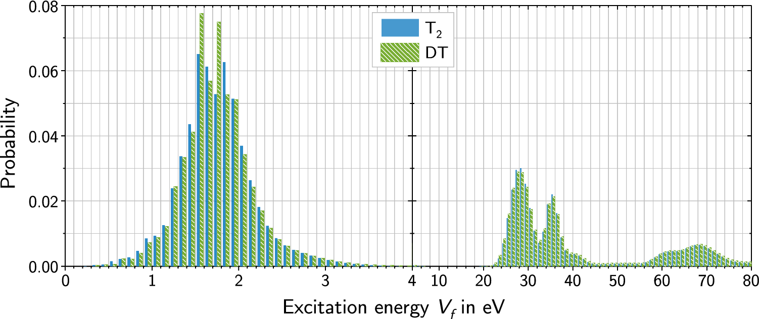
M. Kleesiek et al., EPJ C 79, 204 (2019), Fig. 3, CC BY 4.0.
Tritium
Why Tritium?
\[ {}^3\mathrm H \to{}^3\mathrm{He}^{+}+e^-+\bar\nu_e, \qquad E_0\simeq18.6~\mathrm{keV}. \]
- small \(E_0\): the relative fraction of events near the endpoint is large;
- superallowed transition: the nuclear matrix element hardly changes the shape;
- \(T_{1/2}=12.32\) years: high specific activity and a stable source;
- light system: recoil and molecular states can be computed accurately.
Near the endpoint of the allowed spectrum at \(m_\beta=0\)
\[ \frac{d\Gamma}{dE}\propto(E_0-E)^2. \]
Therefore the fraction of decays in the last interval \(\Delta E\) is estimated as
\[ f(\Delta E) \simeq \frac{\int_{E_0-\Delta E}^{E_0}(E_0-E)^2dE} {\int_0^{E_0}(E_0-E)^2dE} =\left(\frac{\Delta E}{E_0}\right)^3. \]
For \(\Delta E=1~\mathrm{eV}\) this is only
\[ f\sim1.6\cdot10^{-13}. \]
KATRIN uses molecular tritium:
\[ \mathrm T_2\to{}^3\mathrm{HeT}^{+}+e^-+\bar\nu_e. \]
The molecule is convenient to store and to pump continuously, but the daughter ion receives rotational, vibrational, or electronic excitation.
The unmeasured energy \(V_j\) is subtracted from the neutrino energy:
\[ E_{\nu,j}=E_0-E-V_j. \]
Therefore the distribution of final states enters the spectrum model directly.
From 30 eV to KATRIN
What Did the Experiments of the 1980s Change?
The experiment of V. A. Lyubimov’s group used
- a solid source — a thin film of tritiated valine;
- the Tretyakov magnetic spectrometer with high luminosity;
- a measurement of the shape of the last few hundred electronvolts of the \(\beta\) spectrum.
In 1980 the group reported
\[ m_{\bar\nu_e}\simeq30~\mathrm{eV}. \]
The deficit of electrons near the end of the spectrum was interpreted as a kinematic effect of the neutrino mass.
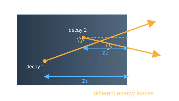
An electron is born at depth \(z\) and leaves at an angle \(\theta\) to the normal. Its path in the material is equal to
\[ \ell=\frac{z}{\cos\theta}, \qquad E_{\mathrm{det}}=E-\Delta E(\ell). \]
Therefore the observed spectrum contains a convolution with the loss distribution \(L\):
\[ S_{\mathrm{obs}}(E) =\int L(\Delta E)S_\beta(E+\Delta E)\,d\Delta E. \]
Non-uniformity of thickness, roughness, and the composition of the film change \(L(\Delta E)\). An error in this function distorts the end of the spectrum and can mimic a mass.
The result was checked in Los Alamos, Zurich, Mainz, and Troitsk. A mass of about \(30~\mathrm{eV}\) was not confirmed.
The main lesson: energy resolution alone is not enough. The end of the spectrum is distorted by effects that resemble a mass:
\[ \text{energy losses} +\text{final states} +\text{response function}. \]
The source and the spectrometer must be calibrated and modeled together.
The next generation combined
\[ \boxed{\text{windowless gas source }\mathrm T_2} \qquad+\qquad \boxed{\text{MAC-E filter}}. \]
A gaseous source eliminates the substrate. The MAC-E filter combines a large solid angle with sub-eV energy resolution.
This combination was developed in Mainz and Troitsk and scaled up in KATRIN.
Exercises for this lecture
- 4.1. Spectrum of \(\beta\) decay
- 4.2. Effective mass and the Kurie plot
- 4.3. Coulomb focusing and the Fermi function
- 4.4. How the Fermi function changes the \(\beta^-\) and \(\beta^+\) spectra
- 4.5. Film, energy losses, and a false neutrino mass
- 4.6. Kink from a heavy mass state
- 4.7. What can \(m_\beta\) be?
- 4.8. Nuclear recoil and the endpoint of the tritium spectrum
- 4.9. How many decays are needed to see the mass?
All exercises for lecture 04 → and exercises for the seminar · All course exercises