Neutrinos. First Contact
Introduction to Neutrino Physics
JINR
Before We Begin
Basic Courses
This lecture requires the basic ideas from three branches of physics:
- special relativity;
- quantum mechanics;
- classical field theory.
The materials of the corresponding courses are available at teach-in.ru.
Natural Units
We set
\[ \hbar=c=1. \]
Then
\[ [E]=[m]=[L]^{-1}=[t]^{-1}, \]
\[ E^2=\mathbf p^2+m^2, \qquad E=\omega, \qquad ƛ=\frac{1}{p} \qquad t\sim\frac{1}{E}. \]
Useful conversions:
\[ \hbar c=197.327~\mathrm{MeV\,fm}, \]
\[ 1~\mathrm{GeV}^{-1}=0.197~\mathrm{fm}, \]
\[ 1~\mathrm{fm}=5.07~\mathrm{GeV}^{-1}, \]
\[ 1~\mathrm{s}=1.52\cdot10^{24}~\mathrm{GeV}^{-1}. \]
1. Matter
What Is Ordinary Matter Made Of?
Ordinary matter needs only two types of fundamental particles:
quarks + electrons
Both quarks and electrons are fermions with spin \(1/2\).
Composite protons and neutrons are also fermions.
2. Interactions
How Do Particles Interact?
Force Carriers
The fundamental interactions are described by the exchange of field quanta — bosons.
| Interaction | Carrier | Spin |
|---|---|---|
| electromagnetic | photon \(\gamma\) | \(1\) |
| weak | \(W^\pm\), \(Z\) | \(1\) |
| strong | gluons \(g\) | \(1\) |
Gravity is not included in the Standard Model of particle physics.
3. Classification of Particles
Fermions and Bosons
Fermions
Half-integer spin: \(1/2, 3/2, \ldots\)
They make up matter.
Bosons
Integer spin: \(0, 1, \ldots\)
They carry interactions; the Higgs field has spin 0.
4. The Standard Model
Particles and the Three Pillars of the Model
Quarks
Leptons
Bosons
- Quantum fields
- Gauge symmetry
\(SU(3)_C\times SU(2)_L\times U(1)_Y\) - Spontaneous symmetry breaking
masses of \(W^\pm\), \(Z\) and fermions
Particles and Fields
The fundamental objects are quantum fields:
- lepton and quark fields are fermionic;
- the fields of the force carriers and the Higgs field are bosonic.
A particle is a quantum of excitation of the corresponding field.
\[ \text{real particle:}\quad E^2=\mathbf p^2+m^2. \]
The internal lines of the diagrams describe virtual states, for which in general
\[ E^2\ne\mathbf p^2+m^2. \]
A Field as a System of Oscillators
A field can be represented as an infinite system of coupled quantum oscillators — one at each point of space.
A Particle as an Excitation of a Field
A particle is a localized excitation of a field, capable of carrying energy, momentum, and quantum numbers.
Analogy: Coupled Oscillators
5. What We Know About Neutrinos
Electric Charge
Theoretically, in the minimal Standard Model
\[ q_\nu=0. \]
But experiment must check whether the neutrino has a very small charge.
Scattering on electrons:
\[ \frac{d\sigma}{dT}\propto\frac{q_\nu^2}{T^2} \quad\Longrightarrow\quad |q_\nu|\lesssim10^{-12}e. \]
Electric neutrality of matter:
\[ n\to p+e^-+\bar\nu_e \]
gives constraints down to
\[ |q_\nu|\lesssim10^{-21}e. \]
Spin
The neutrino is a fermion with spin
\[ s=\frac12. \]
The projection of the spin onto a chosen axis takes two values:
\[ S_z=\pm\frac{\hbar}{2}. \]
We will discuss the helicity and polarization of the neutrino in Lecture 03.
Flavors
Flavor is a quantum number that distinguishes three types of neutrinos:
- \(\nu_e\) — electron neutrino, 1956;
- \(\nu_\mu\) — muon neutrino, 1962;
- \(\nu_\tau\) — tau neutrino, 2000.
In the weak charged current, the neutrino flavor is tied to the charged lepton:
\[ \nu_e+n\to p+e^-, \qquad \nu_\mu+n\not\to p+e^-. \]
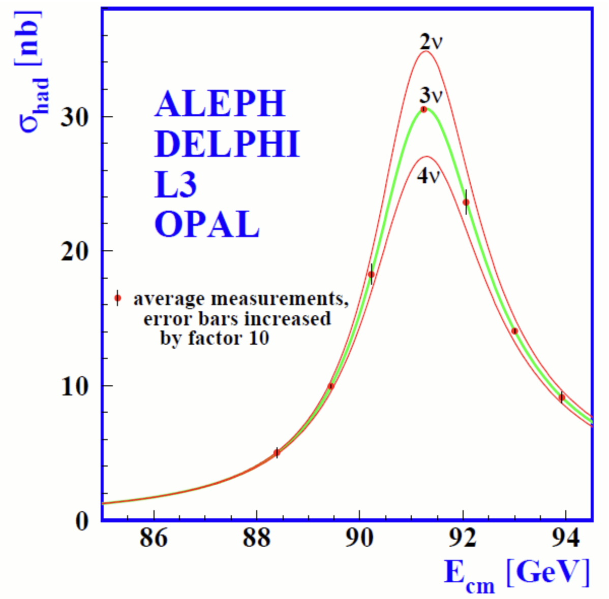
The measurement of the \(Z\)-boson width implies that there are three light active neutrinos.
Mass States
Flavor states do not have a definite mass:
\[ |\nu_\alpha\rangle = \sum_{i=1}^{3}U_{\alpha i}^*|\nu_i\rangle, \qquad \alpha=e,\mu,\tau. \]
- \(\nu_e,\nu_\mu,\nu_\tau\) are produced and detected in the weak interaction;
- \(\nu_1,\nu_2,\nu_3\) propagate with definite masses \(m_1,m_2,m_3\);
- antineutrinos form the corresponding conjugate states.
It is precisely the mismatch between the flavor and mass bases that leads to oscillations.
Neutrino Interactions
- Neutrinos take part in the weak and gravitational interactions.
- At accessible energies, the gravitational interaction of an individual neutrino is negligibly small.
Cross Section and Interaction Length
The probability of traveling a distance \(x\) without interacting is
\[ P_0(x)=e^{-x/\lambda}. \]
The mean interaction length:
\[ \lambda=\frac{1}{n\sigma}, \]
where \(\sigma\) is the cross section and \(n\) is the concentration of targets. For atoms
\[ n_{\rm atom}=\frac{\rho N_A}{A}, \qquad n_e=Z\frac{\rho N_A}{A}. \]
\(\rho\) is the density of the medium, \(A\) is the molar mass, and \(Z\) is the number of electrons in the atom.
Example: Solar Neutrino
For \(E_\nu\sim1~\mathrm{MeV}\) let us estimate the scattering on electrons in the Sun:
\[ \sigma(\nu_e e\to\nu_e e)\sim10^{-44}~\mathrm{cm}^2, \]
\[ n_e\sim \rho N_A\frac{Z}{A} \sim7\cdot10^{23}~\mathrm{cm}^{-3}. \]
Hence
\[ \lambda_\nu \sim\frac{1}{n_e\sigma} \sim10^{20}~\mathrm{cm} \sim10^9R_\odot. \]
The Sun is practically transparent to neutrinos with energies of order MeV.
Example: Neutrino with an Energy of 1 PeV
For passage through the Earth:
\[ \sigma(\nu N)\sim10^{-33}~\mathrm{cm}^2, \]
\[ n_N\sim\rho N_A \sim 5.5~\frac{\mathrm{g}}{\mathrm{cm}^3}, 6.02\cdot10^{23}~\mathrm{g}^{-1} \sim3.3\cdot10^{24}~\mathrm{cm}^{-3}. \]
\[ \lambda_\nu \sim\frac{1}{n_N\sigma} \sim3\cdot10^8~\mathrm{cm} \sim3000~\mathrm{km}. \]
At energies of order PeV, the Earth is already opaque to a significant fraction of neutrinos.
Spatial Parity
The parity transformation reflects space:
\[ P:\quad \mathbf r\to-\mathbf r. \]
The weak interaction does not conserve parity: it singles out left-handed chiral fermions,
\[ J_L^\mu = \bar\psi\gamma^\mu\frac{1-\gamma^5}{2}\psi. \]
This is reflected directly in the gauge group
\[ SU(2)_L\times U(1)_Y. \]
The experimental discovery of parity violation is the topic of Lecture 02.
Neutrinos in the Weak Interaction
In the weak charged current, the three neutrinos form pairs with charged leptons:
\[ \begin{pmatrix}\nu_e\\e\end{pmatrix}_L, \qquad \begin{pmatrix}\nu_\mu\\\mu\end{pmatrix}_L, \qquad \begin{pmatrix}\nu_\tau\\\tau\end{pmatrix}_L. \]
If neutrinos were considered massless, these three flavor states could be treated independently.
But oscillations show that:
\[ \Delta m_{ij}^2\ne0. \]
The Standard Model with Neutrino Masses
Quarks
Leptons
Bosons
In free propagation:
neutrinos have definite masses \(m_1,m_2,m_3\).
In the weak interaction:
the states \(\nu_e,\nu_\mu,\nu_\tau\) are produced and detected.
Mixing of Lepton Generations
The charged weak current contains the Pontecorvo–Maki–Nakagawa–Sakata matrix:
\[ \mathcal L_{\rm CC} = -\frac{g}{\sqrt2} \sum_{\alpha,i} \bar\ell_{\alpha L}\gamma^\mu U_{\alpha i}\nu_{iL}W^-_\mu +\mathrm{h.c.} \]
\[ U_{\rm PMNS} = \begin{pmatrix} U_{e1}&U_{e2}&U_{e3}\\ U_{\mu1}&U_{\mu2}&U_{\mu3}\\ U_{\tau1}&U_{\tau2}&U_{\tau3} \end{pmatrix}, \qquad U^\dagger U=1. \]
The non-diagonal nature of \(U_{\rm PMNS}\) means that the flavor changes as the neutrino propagates.
Neutrino Oscillations
Two Flavors and Two Mass States
In the simplest model
\[ \begin{pmatrix} |\nu_e\rangle\\ |\nu_\mu\rangle \end{pmatrix} = \begin{pmatrix} \cos\theta&-\sin\theta\\ \sin\theta&\cos\theta \end{pmatrix} \begin{pmatrix} |\nu_1\rangle\\ |\nu_2\rangle \end{pmatrix}. \]
Each mass state acquires its own phase as it propagates:
\[ |\nu_i(L)\rangle = e^{-i\phi_i(L)}|\nu_i(0)\rangle. \]
The observed oscillation is the result of interference of these phases.
Probabilities in Vacuum
For two flavors
\[ P(\nu_e\to\nu_e) = 1-\sin^2 2\theta\, \sin^2\!\left(\frac{\Delta m^2L}{4E}\right), \]
\[ P(\nu_e\to\nu_\mu) = \sin^2 2\theta\, \sin^2\!\left(\frac{\Delta m^2L}{4E}\right). \]
Practical form of the phase:
\[ \frac{\Delta m^2L}{4E} = 1.267\, \frac{\Delta m^2[\mathrm{eV}^2]L[\mathrm{km}]}{E[\mathrm{GeV}]}. \]
The Neutrino as a Quantum Chameleon
Experimental Evidence
Oscillations have manifested themselves in independent classes of experiments:
- the deficit of solar electron neutrinos;
- the anomaly in the ratio of atmospheric \(\nu_\mu/\nu_e\);
- the disappearance of reactor antineutrinos;
- the disappearance and appearance of flavors in accelerator beams;
- the dependence of the probabilities on the ratio \(L/E\).
A joint description of all these data requires nonzero
\[ \Delta m_{ij}^2. \]
The Solar Neutrino Flux — Without a Model of the Sun
1. Two neutrinos per cycle
However the individual reactions proceed, their overall result is:
\[ 4p\to{}^4\mathrm{He}+2e^++2\nu_e, \qquad n_\nu=2. \]
The energy release is known from the mass difference
\[ Q\simeq26.7~\mathrm{MeV}. \]
2. The energy flux is measured at the Earth
The solar constant is the luminosity divided by the area of a sphere:
\[ F_\odot\equiv\frac{L_\odot}{4\pi d^2} =1.361~\mathrm{kW\,m^{-2}}. \]
3. We count the number of cycles — and of neutrinos
First, let us convert the “price” of one cycle into joules:
\[ Q=26.7\times10^6\times1.602\times10^{-19} =4.28\times10^{-12}~\mathrm{J}. \]
The number of completed cycles per second per unit area:
\[ \frac{\dot N_{\rm cycle}}{4\pi d^2} =\frac{F_\odot}{Q} =\frac{1.361\times10^3}{4.28\times10^{-12}} =3.18\times10^{14}~\mathrm{m^{-2}\,s^{-1}}. \]
Each cycle yields two neutrinos:
\[ \Phi_\nu=\frac{2F_\odot}{Q} =6.36\times10^{14}~\mathrm{m^{-2}\,s^{-1}} =6.36\times10^{10}~\mathrm{cm^{-2}\,s^{-1}} \approx\boxed{6.5\times10^{10}~\mathrm{cm^{-2}\,s^{-1}}}. \]
This is the strength of the estimate: one needs neither the temperature and density of the solar core, nor the reaction cross sections, nor the branching fractions of the chain. All that is needed is the measured \(F_\odot\), the law of energy conservation, and the fact that two neutrinos are produced per \({}^4\mathrm{He}\) nucleus.
The accuracy of the estimate is a few percent: a small part of \(Q\) is carried away by the neutrinos themselves. The historical deficit was observed in the flux of \(\nu_e\): part of it turned into \(\nu_\mu\) and \(\nu_\tau\) along the way.
Solar Neutrino Experiments
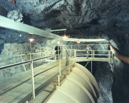
USA
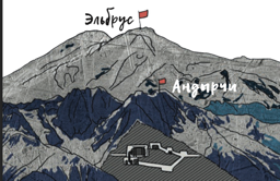
USSR / Russia
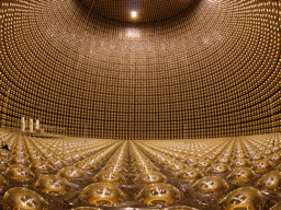
Japan
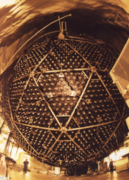
Canada
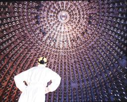
Italy
The results of solar neutrino experiments showed that the flux of electron neutrinos at the Earth is approximately three times smaller than expected. This was the first convincing evidence of neutrino oscillations.
Atmospheric neutrinos
Cosmic rays produce pions in the atmosphere:
\[ p+A\to\text{hadrons}\supset\pi^\pm, \]
\[ \pi^+\to\mu^++\nu_\mu, \qquad \mu^+\to e^++\nu_e+\bar\nu_\mu. \]
Without oscillations, at low energies one expects approximately
\[ \frac{\nu_\mu+\bar\nu_\mu}{\nu_e+\bar\nu_e}\simeq2. \]
The experiment showed that the ratio depends on the distance traveled and on the energy.
6. What we do not yet know
Is CP symmetry violated?
What CP violation means
Charge conjugation replaces a particle with its antiparticle:
\[ C:\quad \text{particle}\to\text{antiparticle}. \]
Parity reflects the coordinates:
\[ P:\quad\mathbf r\to-\mathbf r. \]
CP violation in oscillations would mean
\[ P(\nu_\alpha\to\nu_\beta) \ne P(\bar\nu_\alpha\to\bar\nu_\beta). \]
For example,
\[ P(\nu_\mu\to\nu_e) \ne P(\bar\nu_\mu\to\bar\nu_e). \]
CP phase in the mixing matrix
\[ U_{\rm PMNS} = \underbrace{ \begin{pmatrix} 1&0&0\\0&c_{23}&s_{23}\\0&-s_{23}&c_{23} \end{pmatrix}}_{\text{atmospheric mixing}} \underbrace{ \begin{pmatrix} c_{13}&0&s_{13}e^{-i\delta_{\rm CP}}\\ 0&1&0\\ -s_{13}e^{i\delta_{\rm CP}}&0&c_{13} \end{pmatrix}}_{\text{reactor mixing and }\delta_{\rm CP}} \underbrace{ \begin{pmatrix} c_{12}&s_{12}&0\\-s_{12}&c_{12}&0\\0&0&1 \end{pmatrix}}_{\text{solar mixing}}. \]
Here
\[ s_{ij}=\sin\theta_{ij}, \qquad c_{ij}=\cos\theta_{ij}. \]
The phase \(\delta_{\rm CP}\) is responsible for CP-odd effects in oscillations.
Mass ordering
From solar data it is known that
\[ m_2>m_1, \qquad \Delta m_{21}^2>0. \]
But the sign of the atmospheric mass-squared difference still has to be determined:
Normal ordering
\[ m_1<m_2<m_3. \]
Inverted ordering
\[ m_3<m_1<m_2. \]
Dirac or Majorana?
| Dirac fermion | Majorana fermion | |
|---|---|---|
| Particle and antiparticle | different | identical |
| Example | \(e^-\ne e^+\) | neutrino — possibly |
| Lepton number is conserved | yes | not necessarily |
For an electrically neutral neutrino, both options are possible:
\[ \nu\ne\bar\nu \quad\text{or}\quad \nu=\bar\nu. \]
Observation of neutrinoless double beta decay
\[ (A,Z)\to(A,Z+2)+2e^- \]
would be evidence for the Majorana nature of the neutrino mass.
Absolute mass scale
Mass of the lightest neutrino
Oscillations measure the mass-squared differences:
\[ \Delta m_{ij}^2=m_i^2-m_j^2. \]
They do not determine the overall shift of the mass spectrum.
We do not yet know the mass of the lightest neutrino.
The absolute scale requires kinematic measurements, cosmological observations, or processes that violate lepton number.
Neutrinos as a tool
What can be studied with neutrinos
New physics
rare interactions and unknown particles
The structure of the proton
elastic, inelastic, and deep inelastic scattering
The Sun and stars
reactions in regions inaccessible to photons
Supernovae and the extreme Universe
neutrino telescopes
Nuclear reactors
remote monitoring
The Earth and the Universe
tomography, geoneutrinos, and cosmology
7. Course map
Neutrino theory
Parity, spin, and polarization
Direct determination of the mass
Oscillations in vacuum and in matter
Neutrinos in the Standard Model
Electromagnetic properties and sterile neutrinos
Majorana mass, mixing, and new physics
Sources, interactions, and detectors
Interactions and detection methods
Solar, atmospheric, accelerator, reactor, and geoneutrinos
Relic and ultra-high-energy neutrinos and supernovae
Global data analysis
Neutrino tomography of the Earth
Monitoring of nuclear reactors
Exercises for this lecture
- 1.1. How transparent is the Universe to neutrinos?
- 1.2. Solar neutrino flux
- 1.3. How many light neutrinos exist?
- 1.4. Oscillations of atmospheric neutrinos
- 1.5. Minimal masses for the two level orderings
- 1.6. Dirac or Majorana neutrino?
- 1.7. Where do the cross sections \(10^{-44}\) and \(10^{-33}~\mathrm{cm}^2\) come from?
- 1.8. How neutral is the neutrino?
- 1.9. Why are there twice as many atmospheric \(\nu_\mu\) as \(\nu_e\)?
- 1.10. Why does CP violation need three flavors?
All exercises for lecture 01 → and exercises for the seminar · All course exercises